Some years ago, I spent considerable effort trying to prove the hypothesis below. After failing at this, I spent time trying to find a counterexample, but also with no success. I did post this as a question on mathoverflow, but it has so far received no conclusive answers. So, as far as I am aware, the following statement remains unproven either way.
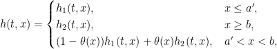
Hypothesis H1 Let  be such that
  is convex in x and right-continuous and decreasing in t. Then, for any semimartingale X,
  is a semimartingale.
It is well known that convex functions of semimartingales are themselves semimartingales. See, for example, the Ito-Tanaka formula. More generally, if was increasing in t rather than decreasing, then it can be shown without much difficulty that is a semimartingale. Consider decomposing as
 |
(1) |
for some process V. By convexity, the right hand derivative of with respect to x always exists, and I am denoting this by  . In the case where f is twice continuously differentiable then the process V is given by Ito’s formula which, in particular, shows that it is a finite variation process. If is convex in x and increasing in t, then the terms in Ito’s formula for V are all increasing and, so, it is an increasing process. By taking limits of smooth functions, it follows that V is increasing even when the differentiability constraints are dropped, so is a semimartingale. Now, returning to the case where is decreasing in t, Ito’s formula is only able to say that V is of finite variation, and is generally not monotonic. As limits of finite variation processes need not be of finite variation themselves, this does not say anything about the case when f is not assumed to be differentiable, and does not help us to determine whether or not is a semimartingale.
Hypothesis H1 can be weakened by restricting to continuous functions of continuous martingales.
Hypothesis H2 Let be such that is convex in x and continuous and decreasing in t. Then, for any continuous martingale X, is a semimartingale.
As continuous martingales are special cases of semimartingales, hypothesis H1 implies H2. In fact, the reverse implication also holds so that hypotheses H1 and H2 are equivalent.
Hypotheses H1 and H2 can also be recast as a simple real analysis statement which makes no reference to stochastic processes.
Hypothesis H3 Let be such that is convex in x and decreasing in t. Then,  where
where  and
and  are convex in x and increasing in t.
Before going any further, I will give some motivation for hypotheses H1 and H2 and explain why it would be good to know whether or not it is true.
Suppose that X is a Markov process and  is such that
  is integrable. Then, we can define a function
 ![{f\colon[0,T]\times{\mathbb R}\rightarrow{\mathbb R}}](https://s0.wp.com/latex.php?latex=%7Bf%5Ccolon%5B0%2CT%5D%5Ctimes%7B%5Cmathbb+R%7D%5Crightarrow%7B%5Cmathbb+R%7D%7D&bg=ffffff&fg=000000&s=0&c=20201002) by
by
![\displaystyle f(t,X_t) = {\mathbb E}[g(X_T)\;\vert\mathcal{F}_t].](https://s0.wp.com/latex.php?latex=%5Cdisplaystyle++f%28t%2CX_t%29+%3D+%7B%5Cmathbb+E%7D%5Bg%28X_T%29%5C%3B%5Cvert%5Cmathcal%7BF%7D_t%5D.+&bg=ffffff&fg=000000&s=0&c=20201002)
This is equivalent to the following two conditions,
-
 .
.
- is a martingale over
 .
.
If we are able to determine which functions f satisfy the martingale condition 2 above, then we can reconstruct the Markov transition function and the distribution of X. For twice differentiable functions, the Kolmogorov backwards equation or Feynman-Kac formula can be used. However, in general, what regularity properties can be imposed on f? It is known that, for diffusions with smoothly defined coefficients, f will be smooth. This does not hold for more general Markov processes. In the case that X is a continuous and strong Markov martingale then, if g is convex, can also be chosen to be convex in x and decreasing in t (see Hobson, Volatility misspecification, option pricing and superreplication via coupling). This is a familiar property in finance, where call and put options have a price which is convex in the underlying asset price and increasing with time to maturity. Although convex and monotonic functions need not be differentiable, the derivatives  and
and  can be interpreted in a measure theoretic sense, and extensions of the backwards equation can be applied. I did post a paper on the arXiv, Fitting Martingales to Given Marginals, using these ideas to show that continuous and strong Markov martingales are uniquely determined by their 1-dimensional marginal distributions (for diffusions with smooth coefficients, this is a well known property of local volatility models used in finance). However, the proof is rather complicated due to the fact that, without knowing hypothesis H1 to be true, it is not even known a-priori whether or not is a semimartingale. Not having a positive answer to hypothesis H1 means that a lot of extra work is required, including the papers Nondifferentiable functions of one-dimensional semimartingales and A Generalized Backward Equation For One Dimensional Processes, which were written in order to develop an alternative technique to get around this obstacle.
Before moving on to the equivalence of the different forms of the hypothesis I will mention that, on balance, I expect that the hypothesis is probably false. As I will show below, it is equivalent to certain sets of integrals being uniformly bounded (H7), and I see no reason for such a bound to exist. However, actually finding examples making these integrals large is difficult, and I still do not have any proven counterexamples to the hypothesis.
I will state various alternative forms of hypothesis H1 in this post and give explanations showing why they are equivalent. For brevity, I do not intend to give complete and rigorous proofs here. However, by filling in the details, all of the arguments can be made fully rigorous. In total I will state nine different forms of the hypothesis, H1 through to H9, and sketch how each of the following implications holds.
Combining these implications shows that all of H1 to H9 are equivalent. In most cases, the reverse implications can also be shown without too much work, the exceptions being H3 ⇒ H1 ⇒ H2. I do not know a quick proof of the converse of these without going all the way round the circle of implications above.
As continuous martingales are special cases of semimartingales, the implication H1 ⇒ H2 is trivial. The implication H3 ⇒ H1 is also straightforward. As argued above, when f is increasing in time, equation (1) decomposes as a stochastic integral plus an increasing process. Hence, whenever decomposes as the difference of functions which are convex in x and increasing in t then (1) expresses as a stochastic integral plus a finite variation process and, if it is also right-continuous, it is a semimartingale.
In hypothesis H3, the terms g and h in the decomposition are given equal status. However, when trying to find such decompositions, I find that it is convenient to regard h as the primary function to be constructed. That is, the problem is to find a function which is convex in x such that  is increasing in t. Then, the function g is defined by
  . Now, restricting to the unit interval
 ![{I=[0,1]}](https://s0.wp.com/latex.php?latex=%7BI%3D%5B0%2C1%5D%7D&bg=ffffff&fg=000000&s=0&c=20201002) , hypothesis H3 can be localized.
, hypothesis H3 can be localized.
Hypothesis H4 Let  be such that is convex and Lipschitz continuous in x and decreasing in t. Then, where and are convex in x and increasing in t.
The idea is that, if f is as in hypothesis H3, then we can apply the decompositions given by H4 on a set of overlapping rectangles covering the right half-plane, and glue these together to obtain the global decomposition. For example, suppose that we have already decomposed  on a rectangle
 ![{[0,T]\times[a,b]}](https://s0.wp.com/latex.php?latex=%7B%5B0%2CT%5D%5Ctimes%5Ba%2Cb%5D%7D&bg=ffffff&fg=000000&s=0&c=20201002) . Then, for any
. Then, for any  apply H4 to obtain the decomposition
  on
on ![{[0,T]\times[a^\prime,b^\prime]}](https://s0.wp.com/latex.php?latex=%7B%5B0%2CT%5D%5Ctimes%5Ba%5E%5Cprime%2Cb%5E%5Cprime%5D%7D&bg=ffffff&fg=000000&s=0&c=20201002) . These can be glued together by choosing a smooth function
. These can be glued together by choosing a smooth function  on the reals such that
  is 0 for
  and 1 for
  . Setting
extends  to the larger rectangle
 ![{[0,T]\times[a,b^\prime]}](https://s0.wp.com/latex.php?latex=%7B%5B0%2CT%5D%5Ctimes%5Ba%2Cb%5E%5Cprime%5D%7D&bg=ffffff&fg=000000&s=0&c=20201002) . It need not be the case that
. It need not be the case that  and
and  are convex in x, but they will have second derivative bounded below and can be made convex by adding a multiple of
  . Continuing in this way, we can extend h to ever larger rectangles to obtain the global decomposition required by H3.
It will be useful to further restrict attention to functions which are equal to zero on the upper and lower edges of the unit rectangle. With this is mind, I make the following definitions.
-
 is the space of functions such that is convex in x and satisfies
  .
.
-
 is the space of
  such that is increasing in t.
-
 is the space of such that is decreasing in t.
In the remainder of the post, for functions of  I will frequently disregard the arguments to keep the expressions reasonably short. I will also use the notation
  and to denote the derivatives of f with respect to its first and second argument respectively. If f is not differentiable, then these can be understood in the sense of distributions. The notation
  will be used for the supremum norm. In particular,
  is finite if and only if f is Lipschitz continuous with respect to x, with Lipschitz constant .
Hypothesis H5 Every  such that
  decomposes as for
  .
.
For any which is convex and Lipschitz continuous in x and decreasing in t, hypothesis H5 can be used to obtain the decomposition stated in H4. By adding a constant to f, without loss of generality we can suppose that  for any
  . We can then extend f to a larger rectangle
 ![{[0,1]\times[-\epsilon,1+\epsilon]}](https://s0.wp.com/latex.php?latex=%7B%5B0%2C1%5D%5Ctimes%5B-%5Cepsilon%2C1%2B%5Cepsilon%5D%7D&bg=ffffff&fg=000000&s=0&c=20201002) by setting
by setting  for x equal to
  and
and  , and linearly interpolating in x across the intervals
  and
and  . So long as
  , this retains convexity in x. Then, hypothesis H5 can be used to decompose and, by restricting to
  , we obtain the decomposition required by hypothesis H4.
Now, if we have a collection  of decompositions (
 ), as in H5, then we can set
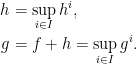
As taking the supremum preserves both convexity in x and monotonicity in t, this gives a decomposition as in H5 with  and
and  for all . Applying this to the collection of all such decompositions gives a maximal decomposition.
Lemma 1 Suppose that is such that the decomposition in (H5) exists. Then, there exists a unique maximal choice for g, h. That is, if is any other such decomposition, then  and
and  .
.
Next, hypothesis H5 is equivalent to the following, apparently weaker, statement.
Hypothesis H6 There exists a constant K such that every with decomposes as for and
 |
(2) |
Clearly, hypothesis H5 follows immediately from H6 simply by dropping (2) from the conclusion. However, H6 does have one advantage — it is only necessary to prove it for a dense subset of . A function is smooth if it is continuous and all of its partial derivates exist, to all orders, on the interior of and extend continuously to . For any , it is not difficult to construct a sequence of smooth  with
with  and converging pointwise to f. So, to prove H6, it is enough to prove it just for smooth functions.
I’ll now describe how to construct the decomposition in H5. This will always converge to the maximal decomposition whenever it exists, or diverge to  if there is no such decomposition. Start by choosing a partition of the unit interval

We now construct  such that is convex in x and is increasing in t. The second condition implies the inequality

Also, from the definition of , we are looking for functions satisfying  . Use
. Use  to denote the convex hull of a function
  . This is the maximum convex function bounded above by u. Then,
  is constructed starting at
  and, then, inductively for
  .
.
 |
(3) |
We can extend h in between the times of the partition however we like, so long as monotonicity in t is preserved. Choosing partitions with mesh  going to zero, we do indeed get convergence to the maximal decomposition whenever it exists.
Lemma 2 Suppose that and, for each  , let
, let  be a partition of the unit interval. We suppose that the partitions have mesh going to 0, and eventually include all times at which f is discontinuous. For each n, let
  be the function constructed as above using the n’th partition. Then, exactly one of the following holds.
- f decomposes as in (H5) and
 pointwise on , where is the maximal decomposition.
- f does not have a decomposition as in (H5), and
 for all
  .
.
Proof: For any given partition, h defined as in (3) is the maximum non-positive function  such that it is convex in x and is increasing in t. This means that
  on
on  whenever the partition
  is a refinement of
  . It follows that

on . Using the fact that the sequence of partitions have mesh going to zero and eventually includes each discontinuity time of f,
So, the constructions along the partitions do converge to a limit, although it could be infinite.
Now, suppose that a decomposition as in H5 does exist. Then, the constructions along partitions are bounded below,  , and must converge to a finite limit. As limits of convex and monotonic functions are, respectively, convex and monotonic, the limit
  is convex in x and
  is increasing in t. As
  , the limit is the maximal decomposition.
Conversely, suppose that there is no such decomposition as in H5. Then, the sequence  cannot converge to a finite limit everywhere. Hence
  for some t and y. By monotonicity in t,
  tends to minus infinity. By convexity, for all
  ,
,
Similarly, the same limit holds for  . ⬜
. ⬜
The construction described above does indeed converge to a finite limit for smooth f.
Lemma 3 Suppose that is smooth. Then, the maximal decomposition exists, the derivative  is bounded, and satisfies
 |
(4) |
Proof: For a given partition of the unit interval, construct h as in (2), and interpolate linearly in between the times of the partition. Setting

then  is the convex hull of
  . The bound

is immediate, where  denotes
  . Hence,
  is bounded by
  . So,
. So,  is bounded by
  . Integrating over t also gives
  .
.
We can also bound  above by
  . Taking its convex hull preserves the bound, so
  is bounded by
  . Similarly,
  is bounded by
  , so
, so  .
.
Next, is bounded below by  and, from this, it can be shown that
  is bounded by
  . So,
. So,  is bounded by
  .
.
Putting all of these together gives the following set of inequalities.
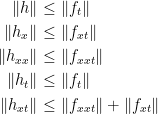 |
(5) |
Now, if is a continuous function with convex hull v, then  and, on each interval for which
  , we have
  . It follows that
  . Applying this to (2) gives
 |
(6) |
We can now take limits as the mesh of the partition goes to zero. The inequality  shows that the construction cannot diverge and, by Lemma 2, the decomposition of hypothesis H5 exists and we have convergence to the maximal decomposition. The inequalities (5) follow for the maximal decomposition and, taking limits of (6) gives

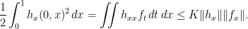
Integrating over and applying integration by parts,

Equality (4) follows from this. ⬜
To construct the decomposition in H5, we can apply the decomposition for smooth f and then take limits to obtain the decomposition for arbitrary . The problem is that, when taking the limit, the terms g and h could diverge to minus infinity. In some cases, (4) can be used to bound h and avoid this potential divergence. However, for this to work, the following alternative version of the hypothesis is required.
Hypothesis H7 There exists a constant K such that all smooth  and
and  satisfy

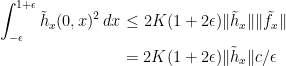
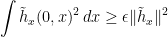
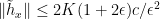
For smooth f, Lemma 3 states that the maximal decomposition as in H5 exists and, assuming hypothesis H7, we have the inequality
If the left hand side can be replaced by a multiple of  then, cancelling
  , this would give inequality (2) as required by hypothesis H6. To do this, we can consider applying the decomposition over a slightly larger region. For any
  , define
  on
on ![{I\times[-\epsilon,1 + \epsilon]}](https://s0.wp.com/latex.php?latex=%7BI%5Ctimes%5B-%5Cepsilon%2C1+%2B+%5Cepsilon%5D%7D&bg=ffffff&fg=000000&s=0&c=20201002) by setting
by setting

This is convex in x so long as . Applying the decomposition given by Lemma 2 to gives a  such that is convex in x,
  is increasing in t and,
The additional factor of  on the right hand side is because we are applying the decomposition over an interval of width rather than the unit interval. Using the fact that
  is linear over the intervals
 ![{[-\epsilon,0]}](https://s0.wp.com/latex.php?latex=%7B%5B-%5Cepsilon%2C0%5D%7D&bg=ffffff&fg=000000&s=0&c=20201002) and
and ![{[1,1+\epsilon]}](https://s0.wp.com/latex.php?latex=%7B%5B1%2C1%2B%5Cepsilon%5D%7D&bg=ffffff&fg=000000&s=0&c=20201002) ,
,
Combining with the previous inequality,
As  on the edges of the rectangle
 ![{I\times[-\epsilon,1+\epsilon]}](https://s0.wp.com/latex.php?latex=%7BI%5Ctimes%5B-%5Cepsilon%2C1%2B%5Cepsilon%5D%7D&bg=ffffff&fg=000000&s=0&c=20201002) , this can be integrated to give
, this can be integrated to give

Restricting to the unit square , this gives a convex non-positive h which is convex in x and such that is increasing in t. Setting  and
and  ,
,

This shows that if hypothesis H7 holds for some constant K, then hypothesis H6 also holds, with constant K replaced by  .
.
Now, I move on to yet another form of the hypothesis. For smooth and , consider defining
![\displaystyle \mu_{[f,g]}(\theta)=\iint (f_{xx}g_t+g_{xx}f_t)\theta\,dt\,dx](https://s0.wp.com/latex.php?latex=%5Cdisplaystyle++%5Cmu_%7B%5Bf%2Cg%5D%7D%28%5Ctheta%29%3D%5Ciint+%28f_%7Bxx%7Dg_t%2Bg_%7Bxx%7Df_t%29%5Ctheta%5C%2Cdt%5C%2Cdx+&bg=ffffff&fg=000000&s=0&c=20201002) |
(7) |
for all smooth  of compact support. If hypothesis H7 is true, then the inequality
![\displaystyle \lvert\mu_{[f,g]}(\theta)\rvert\le 2K\lVert f_x\rVert g_x\rVert \lVert\theta\rVert.](https://s0.wp.com/latex.php?latex=%5Cdisplaystyle++%5Clvert%5Cmu_%7B%5Bf%2Cg%5D%7D%28%5Ctheta%29%5Crvert%5Cle+2K%5ClVert+f_x%5CrVert+g_x%5CrVert+%5ClVert%5Ctheta%5CrVert.+&bg=ffffff&fg=000000&s=0&c=20201002)
would hold. Using integration by parts, ![{\mu_{[f,g]}(\theta)}](https://s0.wp.com/latex.php?latex=%7B%5Cmu_%7B%5Bf%2Cg%5D%7D%28%5Ctheta%29%7D&bg=ffffff&fg=000000&s=0&c=20201002) can be rearranged as
can be rearranged as
![\displaystyle \mu_{[f,g]}(\theta)=\iint\left(f_xg_x\theta_t-f_xg_t\theta_x-f_tg_x\theta_x\right)\,dt\,dx.](https://s0.wp.com/latex.php?latex=%5Cdisplaystyle++%5Cmu_%7B%5Bf%2Cg%5D%7D%28%5Ctheta%29%3D%5Ciint%5Cleft%28f_xg_x%5Ctheta_t-f_xg_t%5Ctheta_x-f_tg_x%5Ctheta_x%5Cright%29%5C%2Cdt%5C%2Cdx.+&bg=ffffff&fg=000000&s=0&c=20201002)
This form has the advantage that it makes sense for all and without imposing any smoothness constraints. By convexity, and  are well-defined bounded functions and, by monotonicity,
  and
and  are well-defined measures (i.e., using Lebesgue-Stieltjes integration). I used this idea in the papers A Generalized Backward Equation For One Dimensional Processes and Fitting Martingales to Given Marginals to derive a martingale condition for where X is a continuous strong Markov martingale, and f is convex in x and decreasing in t, without imposing any differentiability constraints. For our purposes in this post, we just use it for the following form of the hypothesis.
Hypothesis H8 There exists a constant K such that
![\displaystyle \lvert\mu_{[f,g]}(\theta)\rvert\le K\lVert f_x\rVert\lVert g_x\rVert\lVert\theta\rVert](https://s0.wp.com/latex.php?latex=%5Cdisplaystyle++%5Clvert%5Cmu_%7B%5Bf%2Cg%5D%7D%28%5Ctheta%29%5Crvert%5Cle+K%5ClVert+f_x%5CrVert%5ClVert+g_x%5CrVert%5ClVert%5Ctheta%5CrVert+&bg=ffffff&fg=000000&s=0&c=20201002)
for all , and smooth  of compact support.
For smooth and , equation (7) shows that hypothesis H8 is equivalent to

As the terms  and
and  have opposite signs, putting a bound on their sum does not imply any bound on the individual terms. Instead, consider choosing a partition
  , let
, let  be the mid-points, and define and
  by
by

Now, we have  over the intervals
 ![{[s_k,t_k]}](https://s0.wp.com/latex.php?latex=%7B%5Bs_k%2Ct_k%5D%7D&bg=ffffff&fg=000000&s=0&c=20201002) and
and  over the intervals
 ![{[t_{k-1},s_k]}](https://s0.wp.com/latex.php?latex=%7B%5Bt_%7Bk-1%7D%2Cs_k%5D%7D&bg=ffffff&fg=000000&s=0&c=20201002) . So,
. So,

Applying hypothesis H8 to the functions and gives

Taking the limit as the mesh of the partition goes to zero gives the inequality

and hypothesis H7 follows immediately from this.
I now move on to the final form of the hypothesis, which re-introduces the stochastic calculus element.
Hypothesis H9 There exists a constant  such that, for every and continuous martingale
 ![{\{X_t\}_{t\in[0,1]}}](https://s0.wp.com/latex.php?latex=%7B%5C%7BX_t%5C%7D_%7Bt%5Cin%5B0%2C1%5D%7D%7D&bg=ffffff&fg=000000&s=0&c=20201002) with
with  ,
,  has mean variation

In particular, this implies that Y is a quasimartingale. Suppose that hypothesis holds. Given any smooth  with
with  on the interior of and
  , define the function
 ![{C\colon[0,1]\times{\mathbb R}\rightarrow{\mathbb R}_+}](https://s0.wp.com/latex.php?latex=%7BC%5Ccolon%5B0%2C1%5D%5Ctimes%7B%5Cmathbb+R%7D%5Crightarrow%7B%5Cmathbb+R%7D_%2B%7D&bg=ffffff&fg=000000&s=0&c=20201002) by
by

This is convex in x and increasing in t. Now, consider the stochastic differential equation
 |
(8) |
for a Brownian motion W and
We only consider solving (8) up until the first time at which X hits 0 or 1, after which X is constant. If the initial distribution of X is chosen so that
![\displaystyle {\mathbb E}[(X_t-x)_+]=C(t,x)](https://s0.wp.com/latex.php?latex=%5Cdisplaystyle++%7B%5Cmathbb+E%7D%5B%28X_t-x%29_%2B%5D%3DC%28t%2Cx%29+&bg=ffffff&fg=000000&s=0&c=20201002)
for  , then this holds for all
 ![{t\in[0,1]}](https://s0.wp.com/latex.php?latex=%7Bt%5Cin%5B0%2C1%5D%7D&bg=ffffff&fg=000000&s=0&c=20201002) . This is a well known result, used in financial option pricing by the local volatility model, where
. This is a well known result, used in financial option pricing by the local volatility model, where  represents the price of a call option of strike price x and maturity t. For any bounded measurable , the following identities hold,
![\displaystyle \setlength\arraycolsep{2pt} \begin{array}{rl} \displaystyle{\mathbb E}\left[\theta(t,X_t)\right]&\displaystyle=\int_0^1\theta(t,x)C_{xx}(t,x)\,dx\smallskip\\ &\displaystyle= \frac12\int_0^1\theta(t,x)g_{xx}(t,x)\,dx,\medskip\\ \displaystyle{\mathbb E}\left[\int_0^1\theta(s,X_s)\,d[X]_s\right]&\displaystyle=2\iint\theta C_t\,dt\,dx\smallskip\\ &\displaystyle = \iint\theta g_t\,dt\,dx. \end{array}](https://s0.wp.com/latex.php?latex=%5Cdisplaystyle++%5Csetlength%5Carraycolsep%7B2pt%7D+%5Cbegin%7Barray%7D%7Brl%7D+%5Cdisplaystyle%7B%5Cmathbb+E%7D%5Cleft%5B%5Ctheta%28t%2CX_t%29%5Cright%5D%26%5Cdisplaystyle%3D%5Cint_0%5E1%5Ctheta%28t%2Cx%29C_%7Bxx%7D%28t%2Cx%29%5C%2Cdx%5Csmallskip%5C%5C+%26%5Cdisplaystyle%3D+%5Cfrac12%5Cint_0%5E1%5Ctheta%28t%2Cx%29g_%7Bxx%7D%28t%2Cx%29%5C%2Cdx%2C%5Cmedskip%5C%5C+%5Cdisplaystyle%7B%5Cmathbb+E%7D%5Cleft%5B%5Cint_0%5E1%5Ctheta%28s%2CX_s%29%5C%2Cd%5BX%5D_s%5Cright%5D%26%5Cdisplaystyle%3D2%5Ciint%5Ctheta+C_t%5C%2Cdt%5C%2Cdx%5Csmallskip%5C%5C+%26%5Cdisplaystyle+%3D+%5Ciint%5Ctheta+g_t%5C%2Cdt%5C%2Cdx.+%5Cend%7Barray%7D+&bg=ffffff&fg=000000&s=0&c=20201002)
Now, for smooth , (1) expresses  as a martingale plus a finite variation term
![\displaystyle V_t=f(0,X_0) + \frac12\int_0^t f_{xx}(s,X_s)\,d[X]_s + \int_0^t f_t(s,X_s)\,ds.](https://s0.wp.com/latex.php?latex=%5Cdisplaystyle++V_t%3Df%280%2CX_0%29+%2B+%5Cfrac12%5Cint_0%5Et+f_%7Bxx%7D%28s%2CX_s%29%5C%2Cd%5BX%5D_s+%2B+%5Cint_0%5Et+f_t%28s%2CX_s%29%5C%2Cds.+&bg=ffffff&fg=000000&s=0&c=20201002)
Now, using the identities above, for bounded measurable ,
![\displaystyle \setlength\arraycolsep{2pt} \begin{array}{rl} \displaystyle {\mathbb E}\left[\int_0^1\theta(t,X_t)\,dV_t\right]&\displaystyle=\frac12\iint(f_{xx}g_t+g_{xx}f_t)\theta\,dt\,dx\smallskip\\ &\displaystyle=\frac12\mu_{[f,g]}(\theta). \end{array}](https://s0.wp.com/latex.php?latex=%5Cdisplaystyle++%5Csetlength%5Carraycolsep%7B2pt%7D+%5Cbegin%7Barray%7D%7Brl%7D+%5Cdisplaystyle+%7B%5Cmathbb+E%7D%5Cleft%5B%5Cint_0%5E1%5Ctheta%28t%2CX_t%29%5C%2CdV_t%5Cright%5D%26%5Cdisplaystyle%3D%5Cfrac12%5Ciint%28f_%7Bxx%7Dg_t%2Bg_%7Bxx%7Df_t%29%5Ctheta%5C%2Cdt%5C%2Cdx%5Csmallskip%5C%5C+%26%5Cdisplaystyle%3D%5Cfrac12%5Cmu_%7B%5Bf%2Cg%5D%7D%28%5Ctheta%29.+%5Cend%7Barray%7D+&bg=ffffff&fg=000000&s=0&c=20201002)
The left hand side is bounded by the mean variation of Y whenever is bounded by 1 so, if hypothesis H9 holds, it is bounded by  . Scaling g and gives,
![\displaystyle \left\lvert\mu_{[f,g]}(\theta)\right\rvert\le 2K\lVert f_x\rVert \lVert g_x\rVert \rVert\theta\rVert.](https://s0.wp.com/latex.php?latex=%5Cdisplaystyle++%5Cleft%5Clvert%5Cmu_%7B%5Bf%2Cg%5D%7D%28%5Ctheta%29%5Cright%5Crvert%5Cle+2K%5ClVert+f_x%5CrVert+%5ClVert+g_x%5CrVert+%5CrVert%5Ctheta%5CrVert.+&bg=ffffff&fg=000000&s=0&c=20201002)
Approximating arbitrary f and g by smooth functions implies hypothesis H8.
It only remains to show how hypothesis H2 implies H9, which I will do now. This is the most difficult of the implications shown in this post, and I will instead show the contrapositive. That is, supposing that H9 is false, we show that H2 is also false. The idea is to construct a continuous martingale X and ![{f\colon[0,1]\times{\mathbb R}\rightarrow{\mathbb R}}](https://s0.wp.com/latex.php?latex=%7Bf%5Ccolon%5B0%2C1%5D%5Ctimes%7B%5Cmathbb+R%7D%5Crightarrow%7B%5Cmathbb+R%7D%7D&bg=ffffff&fg=000000&s=0&c=20201002) such that the process V in decomposition (1) has infinite variation. This will imply that is not a semimartingale.
such that the process V in decomposition (1) has infinite variation. This will imply that is not a semimartingale.
Start by choosing a sequence of continuous martingales ![{\{X^n\}_{t\in[0,1]}}](https://s0.wp.com/latex.php?latex=%7B%5C%7BX%5En%5C%7D_%7Bt%5Cin%5B0%2C1%5D%7D%7D&bg=ffffff&fg=000000&s=0&c=20201002) with
with  and smooth such that the mean variation of
  is greater than
  . Passing to a larger probability space if necessary, we suppose that we have a doubly indexed sequence
  of independent continuous martingales, where has the same distribution as
  . We then decompose

The variation,  , of
, of  over
over ![{[0,1]}](https://s0.wp.com/latex.php?latex=%7B%5B0%2C1%5D%7D&bg=ffffff&fg=000000&s=0&c=20201002) then has expectation equal to the mean variation of
then has expectation equal to the mean variation of  . By the weak law of large numbers,
with probability at least 1/2, for large enough  . We also suppose that
  . Setting
  for
for  and
and  otherwise. Then,
and  is an integer. Rearranging the non-zero terms gives a singly indexed sequence
  with
with
where  is an integer, are smooth with
  , is an independent sequence of continuous martingales with decomposition

and  has variation
  over .
Let  be the rectangle
 ![{[0,1]\times[-1,1]}](https://s0.wp.com/latex.php?latex=%7B%5B0%2C1%5D%5Ctimes%5B-1%2C1%5D%7D&bg=ffffff&fg=000000&s=0&c=20201002) . By extrapolating
. By extrapolating  and applying a change of variables, we can suppose that
  are continuous martingales with
  and
and  , and
, and  is convex in x and decreasing in t, such that
  on the boundary of and
  at
at  .
.
Now define the sequence of times  . Define the martingale M by

for  . This is a random walk, interpolated by the continuous martingales
  . The times
  are increasing to 1 and,
![\displaystyle {\mathbb E}[M_{t_n}^2]=\sum_{k=1}^n\epsilon_n^2\le1.](https://s0.wp.com/latex.php?latex=%5Cdisplaystyle++%7B%5Cmathbb+E%7D%5BM_%7Bt_n%7D%5E2%5D%3D%5Csum_%7Bk%3D1%7D%5En%5Cepsilon_n%5E2%5Cle1.+&bg=ffffff&fg=000000&s=0&c=20201002)
This is  -bounded so, by martingale convergence, the limit
  exists in and with probability 1, giving a continuous -bounded martingale
 ![{\{M_t\}_{t\in[0,1]}}](https://s0.wp.com/latex.php?latex=%7B%5C%7BM_t%5C%7D_%7Bt%5Cin%5B0%2C1%5D%7D%7D&bg=ffffff&fg=000000&s=0&c=20201002) .
.
The fact that is an integer implies that the support of  is contained in the set
  or
or  for each
  .
.
Define ![{g\colon[0,1]\times{\mathbb R}\rightarrow{\mathbb R}}](https://s0.wp.com/latex.php?latex=%7Bg%5Ccolon%5B0%2C1%5D%5Ctimes%7B%5Cmathbb+R%7D%5Crightarrow%7B%5Cmathbb+R%7D%7D&bg=ffffff&fg=000000&s=0&c=20201002) by
by  for
for  and
and  . We interpolate between these times by setting

for and  , some
  . This is convex in x and decreasing in t. It can be seen that

Then, if we decompose
 |
(9) |
the process V is continuous with variation

This is finite, but tends to infinity almost surely as n goes to infinity.
We can now conclude that  is not a semimartingale as, otherwise, it would decompose uniquely as

for a continuous local martingale N and continuous FV process A with  . Comparing with (9) over each interval
 ![{[0,t]}](https://s0.wp.com/latex.php?latex=%7B%5B0%2Ct%5D%7D&bg=ffffff&fg=000000&s=0&c=20201002) for
for  gives
gives  and, hence, A has almost surely infinite variation on , contradicting the fact that it is an FV process. This then contradicts hypothesis H2.

