Continuous Semimartingales

A stochastic process is a semimartingale if and only if it can be decomposed as the sum of a local martingale and an FV process. This is stated by the Bichteler-Dellacherie theorem or, alternatively, is often taken as the definition of a semimartingale. For continuous semimartingales, which are the subject of this post, things simplify considerably. The terms in the decomposition can be taken to be continuous, in which case they are also unique. As usual, we work with respect to a complete filtered probability space ${(\Omega,\mathcal{F},\{\mathcal{F}_t\}_{t\ge0},{\mathbb P})}$ , all processes are real-valued, and two processes are considered to be the same if they are indistinguishable.

Theorem 1 A continuous stochastic process X is a semimartingale if and only if it decomposes as

$\displaystyle X=M+A$ (1)

for a continuous local martingale M and continuous FV process A. Furthermore, assuming that ${A_0=0}$ , decomposition (1) is unique.

Proof: As sums of local martingales and FV processes are semimartingales, X is a semimartingale whenever it satisfies the decomposition (1). Furthermore, if ${X=M+A=M^\prime+A^\prime}$ were two such decompositions with ${A_0=A^\prime_0=0}$ then ${M-M^\prime=A^\prime-A}$ is both a local martingale and a continuous FV process. Therefore, ${A^\prime-A}$ is constant, so ${A=A^\prime}$ and ${M=M^\prime}$ .

It just remains to prove the existence of decomposition (1). However, X is continuous and, hence, is locally square integrable. So, Lemmas 4 and 5 of the previous post say that we can decompose ${X=M+A}$ where M is a local martingale, A is an FV process and the quadratic covariation ${[M,A]}$ is a local martingale. As X is continuous we have ${\Delta M=-\Delta A}$ so that, by the properties of covariations,

$\displaystyle -[M,A]_t=-\sum_{s\le t}\Delta M_s\Delta A_s=\sum_{s\le t}(\Delta A_s)^2.$

(2)

We have shown that ${-[M,A]}$ is a nonnegative local martingale so, in particular, it is a supermartingale. This gives ${\mathbb{E}[-[M,A]_t]\le\mathbb{E}[-[M,A]_0]=0}$ . Then (2) implies that ${\Delta A}$ is zero and, hence, A and ${M=X-A}$ are continuous. ⬜

Using decomposition (1), it can be shown that a predictable process ${\xi}$ is X-integrable if and only if it is both M-integrable and A-integrable. Then, the integral with respect to X breaks down into the sum of the integrals with respect to M and A. This greatly simplifies the construction of the stochastic integral for continuous semimartingales. The integral with respect to the continuous FV process A is equivalent to Lebesgue-Stieltjes integration along sample paths, and it is possible to construct the integral with respect to the continuous local martingale M for the full set of M-integrable integrands using the Ito isometry. Many introductions to stochastic calculus focus on integration with respect to continuous semimartingales, which is made much easier because of these results.

Theorem 2 Let ${X=M+A}$ be the decomposition of the continuous semimartingale X into a continuous local martingale M and continuous FV process A. Then, a predictable process ${\xi}$ is X-integrable if and only if

$\displaystyle \int_0^t\xi^2\,d[M]+\int_0^t\vert\xi\vert\,\vert dA\vert < \infty$ (3)

almost surely, for each time ${t\ge0}$ . In that case, ${\xi}$ is both M-integrable and A-integrable and,

$\displaystyle \int\xi\,dX=\int\xi\,dM+\int\xi\,dA$ (4)

gives the decomposition of ${\int\xi\,dX}$ into its local martingale and FV terms.

Proof: First, suppose that (3) holds. As ${\int_0^t\xi^2\,d[M]}$ is finite, ${\xi}$ is M-integrable. Also, as ${\int_0^t\vert\xi\vert\,\vert dA\vert}$ is finite, ${\xi}$ is A-integrable and ${\int\xi\,dA}$ agrees with the Lebesgue-Stieltjes integral. As ${\xi}$ is integrable with respect to both M and A, it is integrable with respect to X. By preservation of the local martingale property, the term ${\int\xi\,dM}$ in decomposition (4) is a continuous local martingale. Also, as it agrees with the Lebesgue-Stieltjes integral along sample paths, ${\int\xi\,dA}$ is an FV process.

It still needs to be shown that inequality (3) holds whenever ${\xi}$ is X-integrable. As A is a continuous FV process, it does not contribute to quadratic variations, so ${[X]=[M]}$ . Commuting stochastic integration and quadratic variations,

$\displaystyle \int_0^t\xi^2\,d[M]=\int_0^t\xi^2\,d[X]=\left[\int\xi\,dX\right]_t < \infty.$

So, the first term on the left of (3) is finite.

As ${\int\xi\,dX}$ is a continuous semimartingale, it decomposes as ${N+B}$ for a continuous local martingale N and FV process B, which can be assumed to start from zero. Setting ${\alpha=(1+\vert\xi\vert)^{-1}}$ , the fact that ${\alpha}$ and ${\alpha\xi}$ are bounded predictable processes gives

$\displaystyle \int\alpha\xi\,dM+\int\alpha\xi\,dA=\int\alpha\xi\,dX=\int\alpha\,dN+\int\alpha\,dB.$

Uniqueness of the decomposition into continuous local martingale and FV terms implies that ${\int\alpha\xi\,dA}$ and ${\int\alpha\,dB}$ are equivalent. Let us denote this process by C. Then, applying associativity of integration to the Lebesgue-Stieltjes integrals,

$\displaystyle \int_0^t\,\vert dB\vert = \int_0^t\alpha^{-1}\,\vert dC\vert=\int_0^t\vert\xi\vert\,\vert dA\vert.$

So, the second term on the left of (3) is also finite. ⬜

A particular consequence of Theorem 2 is that, for a continuous FV process A and predictable ${\xi}$ , then ${\xi}$ is A-integrable if and only if it is A-integrable in the Lebesgue-Stieltjes sense. That is, if ${\int_0^t\vert\xi\vert\,\vert dA\vert}$ is finite. Then, the stochastic integral ${\int\xi\,dA}$ agrees with the Lebesgue-Stieltjes integral along the sample paths. So, for continuous FV processes, stochastic integration does not improve upon standard, non-deterministic, Lebesgue-Stieltjes integration. This might not sound very surprising, but it is not true for general FV processes. There exist non-continuous FV processes A and predictable ${\xi}$ which are A-integrable in the stochastic sense, but ${\int\xi\,dA}$ is not well-defined as a Lebesgue-Stieltjes integral (see Failure of Pathwise Integration for FV Processes). It is also possible to give a more direct proof that stochastic integration coincides with Lebesgue-Stieltjes integration for continuous FV processes without relying on (1). This can be done by applying the Jordan decomposition, as I will show below.

Theorem 1 also has the interesting consequence that continuous FV processes are the only semimartingales with zero quadratic variation.

Lemma 3 Let X be a stochastic process. Then, the following are equivalent.

X is a continuous FV process.

X is a semimartingale with zero quadratic variation.

X is a continuous semimartingale such that ${[X,M]=0}$ for all (continuous) local martingales M.

Proof: It was previously shown that all continuous FV processes are semimartingales with zero quadratic variation. Next, if X is a semimartingale with zero quadratic variation then ${(\Delta X)^2=\Delta[X]=0}$ , so X is continuous. Also, the Cauchy-Schwarz inequality gives

$\displaystyle \left\vert[X,M]_t\right\vert\le\sqrt{[X]_t[M]_t}=0$

for all local martingales M. So, it only needs to be shown that, if X is a continuous semimartingale with zero quadratic covariation against all continuous local martingales then it is an FV process. Let ${X=M+A}$ be decomposition (1). As A is an FV process, the quadratic covariation ${[A,M]}$ is zero. Also, by hypothesis, ${[X,M]}$ is zero. So, M is a continuous local martingale with quadratic variation ${[M]=[X-A,M]=0}$ and, hence is constant. Therefore, ${X=M_0+A}$ is an FV process. ⬜

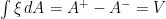
It is also possible to describe integration with respect to continuous FV processes in terms of their Jordan decomposition applied to the sample paths. If A is an FV process, this allows us to write ${A-A_0=A^{+}-A^{-}}$ for increasing processes ${A^+}$ and ${A^-}$ starting from zero. This can be done in such a way that ${A^+}$ and ${A^-}$ are minimal, in which case I refer to them as the increasing and decreasing parts of A respectively. Alternatively, ${A^+}$ and ${A^-}$ are the minimum nonnegative processes such that ${A^+-A}$ and ${A^-+A}$ are increasing. The variation ${V_t}$ of A up until a time t is given by ${V_t=A^+_t+A^-_t}$ . As A is right-continuous, ${A^+,A^-,V}$ are also right-continuous. It can also be seen that they are measurable and adapted by computing them along a partition. Choosing times ${0=t_0\le t_1\le\cdots\le t_n=t}$ then,

$\displaystyle \setlength\arraycolsep{2pt} \begin{array}{rl} \displaystyle V_t &\displaystyle=\lim\sum_{k=1}^n\vert A_{t_k}-A_{t_{k-1}}\vert,\smallskip\\ \displaystyle A^+_t &\displaystyle=\lim\sum_{k=1}^n\left(A_{t_k}-A_{t_{k-1}}\right)_+,\smallskip\\ \displaystyle A^-_t &\displaystyle=\lim\sum_{k=1}^n\left(A_{t_k}-A_{t_{k-1}}\right)_-. \end{array}$

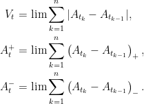The limits here are all taken as ${n\rightarrow\infty}$ and as the mesh of the partition, ${\max_k(t_k-t_{k-1})}$ , goes to zero. So, ${A^+,A^-,V}$ are adapted increasing and right-continuous processes. The Hahn decomposition theorem implies that there exists a measurable process ${\xi}$ with ${\vert\xi\vert=1}$ such that ${\int1_{\{\xi > 0\}}\,dA=A^+}$ , ${-\!\int1_{\{\xi < 0\}}\,dA=A^-}$ and, consequently, ${\int\xi\,dA=V}$ . In general, ${\xi}$ will not be predictable. However, in the case where A is a continuous FV process then ${A^+,A^-,V}$ will be continuous and the following lemma shows that ${\xi}$ can be taken to be predictable.

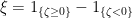
Lemma 4 Let A be a continuous FV process. Then, there exists a predictable process ${\xi}$ with ${\vert\xi\vert=1}$ such that ${\int\xi\,dA}$ is increasing.

Furthermore, if A is any FV process and ${\xi}$ is measurable such that ${\vert\xi\vert=1}$ and ${\int\xi\,dA}$ is increasing, then it follows that ${\int\xi\,dA}$ , ${\int1_{\{\xi > 0\}}\,dA}$ and ${-\!\!\int1_{\{\xi < 0\}}\,dA}$ are respectively the variation, increasing part and decreasing parts of A.

Proof: We start by showing that dA is absolutely continuous with respect to dV. That is, if ${\alpha}$ is a nonnegative bounded predictable process such that ${\int\alpha\,dV=0}$ then we need to show that ${\int\alpha\,dA}$ is zero. As ${V+A=2A^+}$ and ${V-A=2A^-}$ are increasing, this gives

$\displaystyle 0\le 2\int\alpha\,dA^+=\int\alpha\,dA=-2\int\alpha\,dA^-\le0$

so that ${\int\alpha\,dA=0}$ as required. As previously shown, this means that ${A-A_0=\int\zeta\,dV}$ for some predictable process ${\zeta}$ which is V-integrable in the Lebesgue-Stieltjes sense. So, setting ${\xi=1_{\{\zeta\ge0\}}-1_{\{\zeta < 0\}}}$ , we have

$\displaystyle \int\xi\,dA=\int\xi\zeta\,dV=\int\vert\zeta\vert\,dV,$

which is increasing.

Now suppose that A is an FV process, ${\vert\xi\vert=1}$ and that ${\int\xi\,dA}$ is increasing. Integrating ${1_{\{\xi > 0\}}}$ and ${1_{\{\xi < 0\}}}$ with respect to ${\int\xi\,dA}$ shows that the processes ${W\equiv\int1_{\{\xi > 0\}}\,dA}$ and ${W-A=-A_0-\int1_{\{\xi < 0\}}\,dA}$ are increasing. If ${W^\prime}$ was any other increasing process starting from zero such that ${W^\prime-A}$ is increasing then we would have

$\displaystyle W^\prime=\int1_{\{\xi > 0\}}\,d(W^\prime-A)+\int1_{\{\xi < 0\}}\,dW^\prime + W\ge W,$

implying that ${W=A^+}$ as claimed. Applying the same result to ${-A}$ shows that ${-\int1_{\{\xi < 0\}}\,dA=A^-}$ and, therefore, ${\int\xi\,dA=A^+-A^-=V}$ . ⬜

We now give a quick proof that stochastic integration and pathwise Lebesgue-Stieltjes integration coincides for a large class of FV processes, without relying on decomposition (1). The statement of Lemma 5 trivially applies to all increasing FV processes and, applying the lemma above, it also applies to all continuous FV processes.

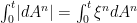
Lemma 5 Let A be an FV process such that ${\int\alpha\,dA}$ is increasing for some bounded predictable and nowhere-zero process ${\alpha}$ .

Then, a predictable process ${\xi}$ is A-integrable if and only if ${\int_0^t\vert\xi\vert\,\vert dA\vert < \infty}$ (almost surely) for each time ${t\ge0}$ . Furthermore, the stochastic and Lebesgue-Stieltjes integrals coincide with probability one.

Proof: Replacing ${\alpha}$ by ${\alpha/\vert\alpha\vert}$ if necessary, we may suppose that ${\vert\alpha\vert=1}$ . Then, Lemma 4 says that ${\int\alpha\,dA}$ is equal to the variation of A. For any A-integrable process ${\xi}$ (in the sense of stochastic integration), choose a sequence of nonnegative bounded predictable processes ${\xi^n}$ increasing to ${\vert\xi\vert}$ . We have

$\displaystyle \setlength\arraycolsep{2pt} \begin{array}{rl} &\displaystyle\int_0^t\vert\xi\vert\,\vert dA\vert =\lim_{n\rightarrow\infty}\int_0^t\xi^n\,\vert dA\vert\smallskip\\ &\displaystyle=\lim_{n\rightarrow\infty}\int_0^t\xi^n\alpha\,dA=\int_0^t\vert\xi\vert\alpha\,dA \end{array}$

The first equality here is just monotone convergence for Lebesgue-Stieltjes integration, and the second equality is substituting ${\int\alpha\,dA}$ for the variation of A. However, as ${\xi^n}$ is bounded, the integral ${\int\xi^n\alpha\,dA}$ is well-defined and identical in the Lebesgue-Stieltjes and stochastic senses. The last equality is dominated convergence for the stochastic integral and, since we know that ${\vert\xi\vert\alpha}$ is A-integrable it follows that ${\int_0^t\vert\xi\vert\,\vert dA\vert}$ is finite. So, ${\xi}$ is A-integrable in the Lebesgue-Stieltjes sense, and the stochastic and Lebesgue-Stieltjes integrals coincide. ⬜

The decomposition of a continuous semimartingale into its local martingale and FV components is quite robust and, in particular, is continuous in the semimartingale topology.

Lemma 6 Let ${\{X^n\}_{n\in{\mathbb N}}}$ , X be continuous local martingales and ${X^n=M^n+A^n}$ , ${X=M+A}$ be their decompositions (1) into continuous local martingale and continuous FV terms with ${A^n_0=A_0=0}$ . Then, the following are equivalent as n goes to infinity.

${X^n\rightarrow X}$ in the semimartingale topology.

${M^n\rightarrow M}$ and ${A^n\rightarrow A}$ in the semimartingale topology.

The following limit holds in probability for each ${t\ge0}$

$\displaystyle (M^n_0-M_0)^2+[M^n-M]_t+\int_0^t\,\vert d(A^n-A)\vert\rightarrow 0.$

Proof: Without loss of generality we can assume that ${X=M=A=0}$ by replacing ${X^n,M^n,A^n}$ with ${X^n-X,M^n-M,A^n-A}$ respectively, if necessary.

Starting with the third condition, by lemma 6 of the post on continuous local martingales, this implies that ${M^n\rightarrow0}$ in the semimartingale topology. Furthermore, for any sequence ${\xi^n}$ of elementary predictable processes bounded by 1, ${\int\xi^ndA^n}$ is bounded by the variation of A up to time t, which tends to zero in probability. So, by definition, ${A^n\rightarrow0}$ in the semimartingale topology, giving the second condition.

That the second condition implies the first is clear from the definition of semimartingale convergence, which is actually a vector topology.

Finally, suppose that the first condition holds. As convergence in the semimartingale topology in particular implies convergence in probability at each time, we see that ${M^n_0=X^n_0}$ tends to zero in probability By the continuity of quadratic variations in the semimartingale topology, ${[M^n]_t=[X^n]_t}$ tends to zero in probability. So, again applying lemma 6 of the post on continuous local martingales, this shows that, under the semimartingale topology, ${M^n\rightarrow0}$ and, hence, ${A^n\rightarrow0}$ . By lemma 4, there exists a sequence ${\xi^n}$ of predictable processes bounded by 1 such that ${\int\xi^ndA^n}$ is equal to the variation of A. Then, by semimartingale convergence, it follows that ${\int_0^t\lvert dA^n\rvert=\int_0^t\xi^ndA^n}$ tends to zero in probability, giving the third statement. ⬜

We previously saw that stochastic integration satisfies dominated convergence, where the integrals of a dominated sequence of integrals converges in the semimartingale topology. For continuous semimartingales, a weaker condition than dominated convergence can be used, and we obtain an ‘if and only if’ condition for the integral to converge.

Theorem 7 Let X be a continuous local martingale and ${X=M+A}$ be decomposition (1). Then, if ${\{\xi^n\}_{n\in{\mathbb N}}}$ and ${\xi}$ are X-integrable processes.

Then, ${\int\xi^n\,dX\rightarrow\int\xi\,dX}$ in the semimartingale topology if and only if

$\displaystyle \int_0^t(\xi^n-\xi)^2\,d[M]+\int_0^t\vert\xi^n-\xi\vert\,\vert dA\vert\rightarrow 0$ (5)

in probability for each t.

Proof: Let use set ${Y=\int\xi dX}$ and ${Y^n=\int\xi^n dX}$ . As integration preserves the semimartingale decomposition, (4), applying theorem 6 with the identity

$\displaystyle \left[\int\xi^n dM-\int\xi dM\right]_t=\int_0^t(\xi^n-\xi)^2d[M]$

shows that ${Y^n\rightarrow Y}$ in the semimartingale topology if and only if (5) tends to zero in probability. ⬜

Ito Processes

Stochastic integration, as originally developed by Kiyoshi Ito, gave a rigorous construction of the integral ${\int\xi\,dB}$ for a predictable process ${\xi}$ and Brownian motion B. Combining this with the standard Lebesgue integral with respect to time leads us to consider processes of the form

$\displaystyle X=X_0+\int\alpha\,dB+\int\beta_s\,ds.$

(6)

Here, B is a Brownian motion defined on the underlying filtered probability space and ${\alpha}$ , ${\beta}$ are predictable processes. For this expression to be well defined, we require ${\int_0^t\alpha_s^2\,ds}$ and ${\int_0^t\vert\beta_s\vert\,ds}$ to be almost surely finite for all times t. Processes of the form (6) are known as Ito processes.

According to this definition, being constructed as integrals with respect to Brownian motion, Ito processes can appear to be a very specialized type of process. However, it turns out that they are surprisingly general and all semimartingales which are absolutely continuous (in the appropriate sense) are Ito processes. This can be proven as a consequence of Lévy’s characterisation of Brownian motion.

Theorem 8 Let X be a continuous stochastic process, and suppose that there exists at least one Brownian motion defined on the underlying filtered probability space. Then the following are equivalent.

X is a semimartingale such that ${\int\xi\,dX=0}$ for all bounded predictable processes ${\xi}$ satisfying ${\int\xi_s\,ds=0}$ .

X satisfies decomposition (6) for some Brownian motion B and predictable processes ${\alpha,\beta}$ satisfying

$\displaystyle \int_0^t\left(\alpha^2_s+\vert\beta_s\vert\right)\,ds < \infty$

(almost surely) for each ${t\ge0}$ .

Proof: First, suppose that X satisfies decomposition (6) and that ${\xi}$ is a bounded predictable process with ${\int\xi_s\,ds=0}$ . Then, integrating ${\beta}$ with respect to ${\int\xi_s\,ds}$ shows that ${\int\xi_s\beta_s\,ds}$ is zero. So, ${\int\xi\,dX=\int\xi\alpha\,dB}$ is a local martingale with quadratic variation ${\int\xi^2\alpha^2\,d[B]=\int\xi^2_s\alpha^2_s\,ds}$ , which is zero. Therefore, ${\int\xi\,dX}$ is constant and, hence, is zero.

Conversely, suppose that the first condition is satisfied. By Theorem 1, we can write ${X=M+A}$ for a continuous local martingale M and continuous FV process A. If ${\xi}$ is a bounded predictable process with ${\int\xi_s\,ds=0}$ then, as continuous FV processes have zero quadratic variation,

$\displaystyle \int\xi^2\,d[M]=\left[\int\xi\,dM\right]=\left[\int\xi\,dX\right]=0.$

As previously shown in the post on Lévy’s characterization, this implies that there exists a Brownian motion B and a predictable process ${\alpha}$ with ${\int_0^t\alpha_s^2\,ds <\infty}$ (for all t) such that ${M=M_0+\int\alpha\,dB}$ . It is here that we needed to assume the existence of at least one Brownian motion on the underlying filtered probability space.

Again, supposing that ${\xi}$ is a bounded predictable process such that ${\int\xi_s\,ds=0}$ then,

$\displaystyle \int\xi\,dA = \int\xi\,dX-\int\xi\,dM = 0.$

As previously shown, this implies that there exists a predictable process ${\beta}$ with ${\int_0^t\vert\beta_s\vert\,ds < \infty}$ (for each t) and such that ${A=A_0+\int\beta_s\,ds}$ . Therefore, decomposition (6) is satisfied. ⬜

Integration with respect to Ito processes reduces to integration with respect to Brownian motion and Lebesgue-Stieltjes integration, by associativity of integration.

Theorem 9 Suppose that X satisfies decomposition (6). Then, a predictable process ${\xi}$ is X-integrable if and only if

$\displaystyle \int_0^t\left(\xi^2_s\alpha^2_s+\vert\xi_s\beta_s\vert\right)\,ds < \infty$ (7)

(almost surely) for all times ${t\ge0}$ . In that case, the integral of ${\xi}$ with respect to X is given by

$\displaystyle \int\xi\,dX=\int\xi\alpha\,dB+\int\xi_s\beta_s\,ds.$

Proof: Writing ${M=\int\alpha\,dB}$ and ${A=\int\beta_s\,ds}$ , Theorem 2 says that ${\xi}$ is X-integrable if and only if

$\displaystyle \int_0^t\xi^2\,d[M]+\int_0^t\vert\xi\vert\,\vert dA\vert = \int_0^t\xi^2\alpha^2\,d[B]+\int_0^t\vert\xi_s\beta_s\vert\,ds$

is finite for each time t. This is equivalent to (7) as Brownian motion has quadratic variation ${[B]_s=s}$ . So, ${\xi}$ is both M and A-integrable and associativity of stochastic integration gives

$\displaystyle \int\xi\,dX=\int\xi\,dM+\int\xi\,dA=\int\xi\alpha\,dB+\int\xi_s\beta_s\,ds$

as required. ⬜

4 thoughts on “Continuous Semimartingales”

Anonymous says:

26 April 15 at 8:06 PM

martingale

Anonymous says:

14 March 17 at 7:08 PM

Hi George,

Thanks for the great blog! During my study of general semimartingale theory, I often encounter the notion of Dirichlet process, a strict superset of the set of semimartingales. Is it possible that you write something on this subject? Namely, I was curious if one can develop theory of stochastic integration w.r.t. Dirichlet process. In addition, I was also curious if there is any simple characterization of Dirichlet processes( except that they are sum of local martingale and zero-energy process). I would like to know if every continuous adapted processes which are martingales under its natural filtration will be Dirichlet.
Thanks in advance and looking forward to your reply!

1. AnastasisKratsios says:
  
  28 June 17 at 9:47 PM
  
  Hi George,
  The following thesis deals with an Ito calculus for Dirichlet processes (using non-anticipative functionals and not only functions)
  
  Click to access fournie.pdf
  
  Enjoy!!
  
zhengxq says:

11 September 17 at 3:56 AM

Hi George,I　love your blog! I am wondering how does the quadratic varition of continuous semimartingales relate to the increasing process in the Doob-Meyer decomposition, which is also called the quadratic variation? Thanks a lot!

	Tavin on Class (D) Processes
	George Lowther on Filtrations and Adapted P…
	faceet on Filtrations and Adapted P…
	George Lowther on Filtrations and Adapted P…
	facet on Filtrations and Adapted P…
	Zoltan on Class (D) Processes
	Zoltan on Class (D) Processes
	ARS on Stopping Times and the Debut…
	George Lowther on Upcrossings, Downcrossings, an…
	George Lowther on Stopping Times and the Debut…

Continuous Semimartingales

Ito Processes

Published by George Lowther

4 thoughts on “Continuous Semimartingales”

Leave a Reply Cancel reply

Ito Processes

Like this:

Related

Published by George Lowther

4 thoughts on “Continuous Semimartingales”

Leave a Reply Cancel reply