Local Time Continuity

Local time surface — Figure 1: Brownian motion and its local time surface

The local time of a semimartingale at a level x is a continuous increasing process, giving a measure of the amount of time that the process spends at the given level. As the definition involves stochastic integrals, it was only defined up to probability one. This can cause issues if we want to simultaneously consider local times at all levels. As x can be any real number, it can take uncountably many values and, as a union of uncountably many zero probability sets can have positive measure or, even, be unmeasurable, this is not sufficient to determine the entire local time ‘surface’

$\displaystyle (t,x)\mapsto L^x_t(\omega)$

for almost all ${\omega\in\Omega}$ . This is the common issue of choosing good versions of processes. In this case, we already have a continuous version in the time index but, as yet, have not constructed a good version jointly in the time and level. This issue arose in the post on the Ito–Tanaka–Meyer formula, for which we needed to choose a version which is jointly measurable. Although that was sufficient there, joint measurability is still not enough to uniquely determine the full set of local times, up to probability one. The ideal situation is when a version exists which is jointly continuous in both time and level, in which case we should work with this choice. This is always possible for continuous local martingales.

Theorem 1 Let X be a continuous local martingale. Then, the local times

$\displaystyle (t,x)\mapsto L^x_t$

have a modification which is jointly continuous in x and t. Furthermore, this is almost surely ${\gamma}$ -Hölder continuous w.r.t. x, for all ${\gamma < 1/2}$ and over all bounded regions for t.

Continue reading “Local Time Continuity” →

Properties of the Dual Projections

In the previous post I introduced the definitions of the dual optional and predictable projections, firstly for processes of integrable variation and, then, generalised to processes which are only required to be locally (or prelocally) of integrable variation. We did not look at the properties of these dual projections beyond the fact that they exist and are uniquely defined, which are significant and important statements in their own right.

To recap, recall that an IV process, A, is right-continuous and such that its variation

$\displaystyle V_t\equiv \lvert A_0\rvert+\int_0^t\,\lvert dA\rvert$

(1)

is integrable at time ${t=\infty}$ , so that ${{\mathbb E}[V_\infty] < \infty}$ . The dual optional projection is defined for processes which are prelocally IV. That is, A has a dual optional projection ${A^{\rm o}}$ if it is right-continuous and its variation process is prelocally integrable, so that there exist a sequence ${\tau_n}$ of stopping times increasing to infinity with ${1_{\{\tau_n > 0\}}V_{\tau_n-}}$ integrable. More generally, A is a raw FV process if it is right-continuous with almost-surely finite variation over finite time intervals, so ${V_t < \infty}$ (a.s.) for all ${t\in{\mathbb R}^+}$ . Then, if a jointly measurable process ${\xi}$ is A-integrable on finite time intervals, we use

$\displaystyle \xi\cdot A_t\equiv\xi_0A_0+\int_0^t\xi\,dA$

to denote the integral of ${\xi}$ with respect to A over the interval ${[0,t]}$ , which takes into account the value of ${\xi}$ at time 0 (unlike the integral ${\int_0^t\xi\,dA}$ which, implicitly, is defined on the interval ${(0,t]}$ ). In what follows, whenever we state that ${\xi\cdot A}$ has any properties, such as being IV or prelocally IV, we are also including the statement that ${\xi}$ is A-integrable so that ${\xi\cdot A}$ is a well-defined process. Also, whenever we state that a process has a dual optional projection, then we are also implicitly stating that it is prelocally IV.

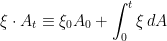
From theorem 3 of the previous post, the dual optional projection ${A^{\rm o}}$ is the unique prelocally IV process satisfying

$\displaystyle {\mathbb E}[\xi\cdot A^{\rm o}_\infty]={\mathbb E}[{}^{\rm o}\xi\cdot A_\infty]$

for all measurable processes ${\xi}$ with optional projection ${{}^{\rm o}\xi}$ such that ${\xi\cdot A^{\rm o}}$ and ${{}^{\rm o}\xi\cdot A}$ are IV. Equivalently, ${A^{\rm o}}$ is the unique optional FV process such that

$\displaystyle {\mathbb E}[\xi\cdot A^{\rm o}_\infty]={\mathbb E}[\xi\cdot A_\infty]$

for all optional ${\xi}$ such that ${\xi\cdot A}$ is IV, in which case ${\xi\cdot A^{\rm o}}$ is also IV so that the expectations in this identity are well-defined.

I now look at the elementary properties of dual optional projections, as well as the corresponding properties of dual predictable projections. The most important property is that, according to the definition just stated, the dual projection exists and is uniquely defined. By comparison, the properties considered in this post are elementary and relatively easy to prove. So, I will simply state a theorem consisting of a list of all the properties under consideration, and will then run through their proofs. Starting with the dual optional projection, the main properties are listed below as Theorem 1.

Note that the first three statements are saying that the dual projection is indeed a linear projection from the prelocally IV processes onto the linear subspace of optional FV processes. As explained in the previous post, by comparison with the discrete-time setting, the dual optional projection can be expressed, in a non-rigorous sense, as taking the optional projection of the infinitesimal increments,

$\displaystyle dA^{\rm o}={}^{\rm o}dA.$

(2)

As ${dA}$ is interpreted via the Lebesgue-Stieltjes integral ${\int\cdot\,dA}$ , it is a random measure rather than a real-valued process. So, the optional projection of ${dA}$ appearing in (2) does not really make sense. However, Theorem 1 does allow us to make sense of (2) in certain restricted cases. For example, if A is differentiable so that ${dA=\xi\,dt}$ for a process ${\xi}$ , then (9) below gives ${dA={}^{\rm o}\xi\,dt}$ . This agrees with (2) so long as ${{}^{\rm o}(\xi\,dt)}$ is interpreted to mean ${{}^{\rm o}\xi\,dt}$ . Also, restricting to the jump component of the increments, ${\Delta A=A-A_-}$ , (2) reduces to (11) below.

We defined the dual projection via expectations of integrals ${\xi\cdot A}$ with the restriction that this is IV. An alternative approach is to first define the dual projections for IV processes, as was done in theorems 1 and 2 of the previous post, and then extend to (pre)locally IV processes by localisation of the projection. That this is consistent with our definitions follows from the fact that (pre)localisation commutes with the dual projection, as stated in (10) below.

Theorem 1

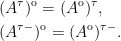
A raw FV process A is optional if and only if ${A^{\rm o}}$ exists and is equal to A.

If the dual optional projection of A exists then,

$\displaystyle (A^{\rm o})^{\rm o}=A^{\rm o}.$ (3)

If the dual optional projections of A and B exist, and ${\lambda}$ , ${\mu}$ are ${\mathcal F_0}$ -measurable random variables then,

$\displaystyle (\lambda A+\mu B)^{\rm o}=\lambda A^{\rm o}+\mu B^{\rm o}.$ (4)

If the dual optional projection ${A^{\rm o}}$ exists then ${{\mathbb E}[\lvert A_0\rvert\,\vert\mathcal F_0]}$ is almost-surely finite and

$\displaystyle A^{\rm o}_0={\mathbb E}[A_0\,\vert\mathcal F_0].$ (5)

If U is a random variable and ${\tau}$ is a stopping time, then ${U1_{[\tau,\infty)}}$ is prelocally IV if and only if ${{\mathbb E}[1_{\{\tau < \infty\}}\lvert U\rvert\,\vert\mathcal F_\tau]}$ is almost surely finite, in which case

$\displaystyle \left(U1_{[\tau,\infty)}\right)^{\rm o}={\mathbb E}[1_{\{\tau < \infty\}}U\,\vert\mathcal F_\tau]1_{[\tau,\infty)}.$ (6)

If the prelocally IV process A is nonnegative and increasing then so is ${A^{\rm o}}$ and,

$\displaystyle {\mathbb E}[\xi\cdot A^{\rm o}_\infty]={\mathbb E}[{}^{\rm o}\xi\cdot A_\infty]$ (7)

for all nonnegative measurable ${\xi}$ with optional projection ${{}^{\rm o}\xi}$ . If A is merely increasing then so is ${A^{\rm o}}$ and (7) holds for nonnegative measurable ${\xi}$ with ${\xi_0=0}$ .

If A has dual optional projection ${A^{\rm o}}$ and ${\xi}$ is an optional process such that ${\xi\cdot A}$ is prelocally IV then, ${\xi}$ is ${A^{\rm o}}$ -integrable and,

$\displaystyle (\xi\cdot A)^{\rm o}=\xi\cdot A^{\rm o}.$ (8)

If A is an optional FV process and ${\xi}$ is a measurable process with optional projection ${{}^{\rm o}\xi}$ such that ${\xi\cdot A}$ is prelocally IV then, ${{}^{\rm o}\xi}$ is A-integrable and,

$\displaystyle (\xi\cdot A)^{\rm o}={}^{\rm o}\xi\cdot A.$ (9)

If A has dual optional projection ${A^{\rm o}}$ and ${\tau}$ is a stopping time then,

$\displaystyle \setlength\arraycolsep{2pt} \begin{array}{rl} &\displaystyle(A^{\tau})^{\rm o}=(A^{\rm o})^{\tau},\smallskip\\ &\displaystyle(A^{\tau-})^{\rm o}=(A^{\rm o})^{\tau-}. \end{array}$ (10)

If the dual optional projection ${A^{\rm o}}$ exists, then its jump process is the optional projection of the jump process of A,

$\displaystyle \Delta A^{\rm o}={}^{\rm o}\!\Delta A.$ (11)

If A has dual optional projection ${A^{\rm o}}$ then

$\displaystyle \setlength\arraycolsep{2pt} \begin{array}{rl} &\displaystyle{\mathbb E}\left[\xi_0\lvert A^{\rm o}_0\rvert + \int_0^\infty\xi\,\lvert dA^{\rm o}\rvert\right]\le{\mathbb E}\left[{}^{\rm o}\xi_0\lvert A_0\rvert + \int_0^\infty{}^{\rm o}\xi\,\lvert dA\rvert\right],\smallskip\\ &\displaystyle{\mathbb E}\left[\xi_0(A^{\rm o}_0)_+ + \int_0^\infty\xi\,(dA^{\rm o})_+\right]\le{\mathbb E}\left[{}^{\rm o}\xi_0(A_0)_+ + \int_0^\infty{}^{\rm o}\xi\,(dA)_+\right],\smallskip\\ &\displaystyle{\mathbb E}\left[\xi_0(A^{\rm o}_0)_- + \int_0^\infty\xi\,(dA^{\rm o})_-\right]\le{\mathbb E}\left[{}^{\rm o}\xi_0(A_0)_- + \int_0^\infty{}^{\rm o}\xi\,(dA)_-\right], \end{array}$ (12)

for all nonnegative measurable ${\xi}$ with optional projection ${{}^{\rm o}\xi}$ .

Let ${\{A^n\}_{n=1,2,\ldots}}$ be a sequence of right-continuous processes with variation
$\displaystyle V^n_t=\lvert A^n_0\rvert + \int_0^t\lvert dA^n\rvert.$

If ${\sum_n V^n}$ is prelocally IV then,

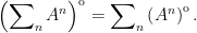$\displaystyle \left(\sum\nolimits_n A^n\right)^{\rm o}=\sum\nolimits_n\left(A^n\right)^{\rm o}.$ (13)

Continue reading “Properties of the Dual Projections” →

Failure of the Martingale Property For Stochastic Integration

If X is a cadlag martingale and ${\xi}$ is a uniformly bounded predictable process, then is the integral

$\displaystyle Y=\int\xi\,dX$

(1)

a martingale? If ${\xi}$ is elementary this is one of most basic properties of martingales. If X is a square integrable martingale, then so is Y. More generally, if X is an ${L^p}$ -integrable martingale, any ${p > 1}$ , then so is Y. Furthermore, integrability of the maximum ${\sup_{s\le t}\lvert X_s\rvert}$ is enough to guarantee that Y is a martingale. Also, it is a fundamental result of stochastic integration that Y is at least a local martingale and, for this to be true, it is only necessary for X to be a local martingale and ${\xi}$ to be locally bounded. In the general situation for cadlag martingales X and bounded predictable ${\xi}$ , it need not be the case that Y is a martingale. In this post I will construct an example showing that Y can fail to be a martingale. Continue reading “Failure of the Martingale Property For Stochastic Integration” →

Purely Discontinuous Semimartingales

As stated by the Bichteler-Dellacherie theorem, all semimartingales can be decomposed as the sum of a local martingale and an FV process. However, as the terms are only determined up to the addition of an FV local martingale, this decomposition is not unique. In the case of continuous semimartingales, we do obtain uniqueness, by requiring the terms in the decomposition to also be continuous. Furthermore, the decomposition into continuous terms is preserved by stochastic integration. Looking at non-continuous processes, there does exist a unique decomposition into local martingale and predictable FV processes, so long as we impose the slight restriction that the semimartingale is locally integrable.

In this post, I look at another decomposition which holds for all semimartingales and, moreover, is uniquely determined. This is the decomposition into continuous local martingale and purely discontinuous terms which, as we will see, is preserved by the stochastic integral. This is distinct from each of the decompositions mentioned above, except for the case of continuous semimartingales, in which case it coincides with the sum of continuous local martingale and FV components. Before proving the decomposition, I will start by describing the class of purely discontinuous semimartingales which, although they need not have finite variation, do have many of the properties of FV processes. In fact, they comprise precisely of the closure of the set of FV processes under the semimartingale topology. The terminology can be a bit confusing, and it should be noted that purely discontinuous processes need not actually have any discontinuities. For example, all continuous FV processes are purely discontinuous. For this reason, the term `quadratic pure jump semimartingale’ is sometimes used instead, referring to the fact that their quadratic variation is a pure jump process. Recall that quadratic variations and covariations can be written as the sum of continuous and pure jump parts,

$\displaystyle \setlength\arraycolsep{2pt} \begin{array}{rl} \displaystyle [X]_t&\displaystyle=[X]^c_t+\sum_{s\le t}(\Delta X_s)^2,\smallskip\\ \displaystyle [X,Y]_t&\displaystyle=[X,Y]^c_t+\sum_{s\le t}\Delta X_s\Delta Y_s. \end{array}$

(1)

The statement that the quadratic variation is a pure jump process is equivalent to saying that its continuous part, ${[X]^c}$ , is zero. As the only difference between the generalized Ito formula for semimartingales and for FV processes is in the terms involving continuous parts of the quadratic variations and covariations, purely discontinuous semimartingales behave much like FV processes under changes of variables and integration by parts. Yet another characterisation of purely discontinuous semimartingales is as sums of purely discontinuous local martingales — which were studied in the previous post — and of FV processes.

Rather than starting by choosing one specific property to use as the definition, I prove the equivalence of various statements, any of which can be taken to define the purely discontinuous semimartingales.

Theorem 1 For a semimartingale X, the following are equivalent.

${[X]^c=0}$ .

${[X,Y]^c=0}$ for all semimartingales Y.

${[X,Y]=0}$ for all continuous semimartingales Y.

${[X,M]=0}$ for all continuous local martingales M.

${X=M+V}$ for a purely discontinuous local martingale M and FV process V.

there exists a sequence ${\{X^n\}_{n=1,2,\ldots}}$ of FV processes such that ${X^n\rightarrow X}$ in the semimartingale topology.

Continue reading “Purely Discontinuous Semimartingales” →

Purely Discontinuous Local Martingales

The previous post introduced the idea of a purely discontinuous local martingale. In the context of that post, such processes were used to construct local martingales with prescribed jumps, and enabled us to obtain uniqueness in the constructions given there. However, purely discontinuous local martingales are a very useful concept more generally in martingale and semimartingale theory, so I will go into more detail about such processes now. To start, we restate the definition from the previous post.

Definition 1 A local martingale X is said to be purely discontinuous iff XM is a local martingale for all continuous local martingales M.

We can show that every local martingale decomposes uniquely into continuous and purely discontinuous parts. Continuous local martingales are well understood — for instance, they can always be realized as time-changed Brownian motions. On the other hand, as we will see in a moment, purely discontinuous local martingales can be realized as limits of FV processes, and arguments involving FV local martingales can often to be extended to the purely discontinuous case. So, decomposition (1) below is useful as it allows arguments involving continuous-time local martingales to be broken down into different approaches involving their continuous and purely discontinuous parts. As always, two processes are considered to be equal if they are equivalent up to evanescence.

Theorem 2 Every local martingale X decomposes uniquely as

$\displaystyle X = X^{\rm c} + X^{\rm d}$ (1)

where ${X^{\rm c}}$ is a continuous local martingale with ${X^{\rm c}_0=0}$ and ${X^{\rm d}}$ is a purely discontinuous local martingale.

Proof: As the process ${H=\Delta X}$ is, by definition, equal to the jump process of a local martingale then it satisfies the hypothesis of Theorem 5 of the previous post. So, there exists a purely discontinuous local martingale ${X^{\rm d}}$ with ${\Delta X^{\rm d}=H=\Delta X}$ . We can take ${X^{\rm d}_0=X_0}$ so that ${X^{\rm c}=X-X^{\rm d}}$ is a continuous local martingale starting from 0.

If ${X=\tilde X^{\rm c}+\tilde X^{\rm d}}$ is another such decomposition, then ${\tilde X^{\rm d}}$ and ${X^{\rm d}}$ have the same jumps and initial value so, by Lemma 3 of the previous post, ${\tilde X^{\rm d}=X^{\rm d}}$ . ⬜

Throughout the remainder of this post, the notation ${X^{\rm c}}$ and ${X^{\rm d}}$ will be used to denote the continuous and purely discontinuous parts of a local martingale X, as given by decomposition (1). Using the notation ${\mathcal{M}_{\rm loc}}$ , ${\mathcal{M}_{{\rm loc},0}^{\rm c}}$ and ${\mathcal{M}_{\rm loc}^{\rm d} }$ respectively for the spaces of local martingales, continuous local martingales starting from zero and the purely discontinuous local martingales, Theorem 2 can be expressed succinctly as

$\displaystyle \mathcal{M}_{\rm loc} = \mathcal{M}_{{\rm loc},0}^{\rm c} \oplus \mathcal{M}_{\rm loc}^{\rm d}.$

(2)

That is, ${\mathcal{M}_{\rm loc}}$ is the direct sum of ${\mathcal{M}_{{\rm loc},0}^{\rm c}}$ and ${\mathcal{M}_{\rm loc}^{\rm d}}$ . Definition 2 identifies the purely discontinuous local martingales to be, in a sense, orthogonal to the continuous local martingales. Then, (2) can be understood as the decomposition of ${\mathcal{M}_{\rm loc}}$ into the direct sum of the closed subspace ${\mathcal{M}_{{\rm loc},0}^{\rm c}}$ and its orthogonal complement. This does in fact give an alternative, elementary, and commonly used, method of proving decomposition (1). As we have already shown the rather strong result of Theorem 5 from the previous post, the quickest way of proving the decomposition was to simply apply this result. I’ll give more details on the more elementary approach further below.

Definition 1 used above for the class of purely discontinuous local martingales was very convenient for our purposes, as it leads immediately to the proof of Theorem 2. However, there are many alternative characterizations of such processes. For example, they are precisely the processes which are limits of FV local martingales in a strong enough sense. They can also be characterized in terms of their quadratic variations and covariations. Recall that the quadratic variation and covariation are FV processes with jumps ${\Delta[X]=(\Delta X)^2}$ and ${\Delta[X,Y]=\Delta X\Delta Y}$ , so that they can be decomposed into continuous and pure jump components,

$\displaystyle \setlength\arraycolsep{2pt} \begin{array}{rl} \displaystyle [X]_t &\displaystyle=[X]^c_t+\sum_{s\le t}(\Delta X_s)^2,\smallskip\\ \displaystyle [X,Y]_t &\displaystyle=[X,Y]^c_t+\sum_{s\le t}\Delta X_s\Delta Y_s. \end{array}$

(3)

The following theorem gives several alternative characterizations of the class of purely discontinuous local martingales.

Theorem 3 For a local martingale X, the following are equivalent.

X is purely discontinuous.

${[X,Y]=0}$ for all continuous local martingales Y.

${[X,Y]^c=0}$ for all local martingales Y.

${[X]^c=0}$ .

there exists a sequence ${\{X^n\}_{n=1,2,\ldots}}$ of FV local martingales such that
$\displaystyle {\mathbb E}\left[\sup_{t\ge0}(X^n_t-X_t)^2\right]\rightarrow0.$

Continue reading “Purely Discontinuous Local Martingales” →

Constructing Martingales with Prescribed Jumps

In this post we will describe precisely which processes can be realized as the jumps of a local martingale. This leads to very useful decomposition results for processes — see Theorem 10 below, where we give a decomposition of a process X into martingale and predictable components. As I will explore further in future posts, this enables us to construct particularly useful decompositions for local martingales and semimartingales.

Before going any further, we start by defining the class of local martingales which will be used to match prescribed jump processes. The purely discontinuous local martingales are, in a sense, the orthogonal complement to the class of continuous local martingales.

Definition 1 A local martingale X is said to be purely discontinuous iff XM is a local martingale for all continuous local martingales M.

The class of purely discontinuous local martingales is often denoted as ${\mathcal{M}_{\rm loc}^{\rm d}}$ . Clearly, any linear combination of purely discontinuous local martingales is purely discontinuous. I will investigate ${\mathcal{M}_{\rm loc}^{\rm d}}$ in more detail later but, in order that we do have plenty of examples of such processes, we show that all FV local martingales are purely discontinuous.

Lemma 2 Every FV local martingale is purely discontinuous.

Proof: If X is an FV local martingale and M is a continuous local martingale then we can compute the quadratic covariation,

$\displaystyle [X,M]_t=\sum_{s\le t}\Delta X_s\Delta M_s=0.$

The first equality follows because X is an FV process, and the second because M is continuous. So, ${XM=XM-[X,M]}$ is a local martingale and X is purely discontinuous. ⬜

Next, an important property of purely discontinuous local martingales is that they are determined uniquely by their jumps. Throughout these notes, I am considering two processes to be equal whenever they are equal up to evanescence.

Lemma 3 Purely discontinuous local martingales are uniquely determined by their initial value and jumps. That is, if X and Y are purely discontinuous local martingales with ${X_0=Y_0}$ and ${\Delta X = \Delta Y}$ , then ${X=Y}$ .

Proof: Setting ${M=X-Y}$ we have ${M_0=0}$ and ${\Delta M = 0}$ . So, M is a continuous local martingale and ${M^2= MX-MY}$ is a local martingale starting from zero. Hence, it is a supermartingale and we have

$\displaystyle {\mathbb E}[M_t^2]\le{\mathbb E}[M_0^2]=0.$

So ${M_t=0}$ almost surely and, by right-continuity, ${M=0}$ up to evanescence. ⬜

Note that if X is a continuous local martingale, then the constant process ${Y_t=X_0}$ has the same initial value and jumps as X. So Lemma 3 has the immediate corollary.

Corollary 4 Any local martingale which is both continuous and purely discontinuous is almost surely constant.

Recalling that the jump process, ${\Delta X}$ , of a cadlag adapted process X is thin, we now state the main theorem of this post and describe precisely those processes which occur as the jumps of a local martingale.

Theorem 5 Let H be a thin process. Then, ${H=\Delta X}$ for a local martingale X if and only if

${\sqrt{\sum_{s\le t}H_s^2}}$ is locally integrable.

${{\mathbb E}[1_{\{\tau < \infty\}}H_\tau\;\vert\mathcal{F}_{\tau-}]=0}$ (a.s.) for all predictable stopping times ${\tau}$ .

Furthermore, X can be chosen to be purely discontinuous with ${X_0=0}$ , in which case it is unique.

Continue reading “Constructing Martingales with Prescribed Jumps” →

Continuous Semimartingales

A stochastic process is a semimartingale if and only if it can be decomposed as the sum of a local martingale and an FV process. This is stated by the Bichteler-Dellacherie theorem or, alternatively, is often taken as the definition of a semimartingale. For continuous semimartingales, which are the subject of this post, things simplify considerably. The terms in the decomposition can be taken to be continuous, in which case they are also unique. As usual, we work with respect to a complete filtered probability space ${(\Omega,\mathcal{F},\{\mathcal{F}_t\}_{t\ge0},{\mathbb P})}$ , all processes are real-valued, and two processes are considered to be the same if they are indistinguishable.

Theorem 1 A continuous stochastic process X is a semimartingale if and only if it decomposes as

$\displaystyle X=M+A$ (1)

for a continuous local martingale M and continuous FV process A. Furthermore, assuming that ${A_0=0}$ , decomposition (1) is unique.

Proof: As sums of local martingales and FV processes are semimartingales, X is a semimartingale whenever it satisfies the decomposition (1). Furthermore, if ${X=M+A=M^\prime+A^\prime}$ were two such decompositions with ${A_0=A^\prime_0=0}$ then ${M-M^\prime=A^\prime-A}$ is both a local martingale and a continuous FV process. Therefore, ${A^\prime-A}$ is constant, so ${A=A^\prime}$ and ${M=M^\prime}$ .

It just remains to prove the existence of decomposition (1). However, X is continuous and, hence, is locally square integrable. So, Lemmas 4 and 5 of the previous post say that we can decompose ${X=M+A}$ where M is a local martingale, A is an FV process and the quadratic covariation ${[M,A]}$ is a local martingale. As X is continuous we have ${\Delta M=-\Delta A}$ so that, by the properties of covariations,

$\displaystyle -[M,A]_t=-\sum_{s\le t}\Delta M_s\Delta A_s=\sum_{s\le t}(\Delta A_s)^2.$

(2)

We have shown that ${-[M,A]}$ is a nonnegative local martingale so, in particular, it is a supermartingale. This gives ${\mathbb{E}[-[M,A]_t]\le\mathbb{E}[-[M,A]_0]=0}$ . Then (2) implies that ${\Delta A}$ is zero and, hence, A and ${M=X-A}$ are continuous. ⬜

Using decomposition (1), it can be shown that a predictable process ${\xi}$ is X-integrable if and only if it is both M-integrable and A-integrable. Then, the integral with respect to X breaks down into the sum of the integrals with respect to M and A. This greatly simplifies the construction of the stochastic integral for continuous semimartingales. The integral with respect to the continuous FV process A is equivalent to Lebesgue-Stieltjes integration along sample paths, and it is possible to construct the integral with respect to the continuous local martingale M for the full set of M-integrable integrands using the Ito isometry. Many introductions to stochastic calculus focus on integration with respect to continuous semimartingales, which is made much easier because of these results.

Theorem 2 Let ${X=M+A}$ be the decomposition of the continuous semimartingale X into a continuous local martingale M and continuous FV process A. Then, a predictable process ${\xi}$ is X-integrable if and only if

$\displaystyle \int_0^t\xi^2\,d[M]+\int_0^t\vert\xi\vert\,\vert dA\vert < \infty$ (3)

almost surely, for each time ${t\ge0}$ . In that case, ${\xi}$ is both M-integrable and A-integrable and,

$\displaystyle \int\xi\,dX=\int\xi\,dM+\int\xi\,dA$ (4)

gives the decomposition of ${\int\xi\,dX}$ into its local martingale and FV terms.

Continue reading “Continuous Semimartingales” →

Zero-Hitting and Failure of the Martingale Property

For nonnegative local martingales, there is an interesting symmetry between the failure of the martingale property and the possibility of hitting zero, which I will describe now. I will also give a necessary and sufficient condition for solutions to a certain class of stochastic differential equations to hit zero in finite time and, using the aforementioned symmetry, infer a necessary and sufficient condition for the processes to be proper martingales. It is often the case that solutions to SDEs are clearly local martingales, but is hard to tell whether they are proper martingales. So, the martingale condition, given in Theorem 4 below, is a useful result to know. The method described here is relatively new to me, only coming up while preparing the previous post. Applying a hedging argument, it was noted that the failure of the martingale property for solutions to the SDE ${dX=X^c\,dB}$ for ${c>1}$ is related to the fact that, for ${c<1}$ , the process hits zero. This idea extends to all continuous and nonnegative local martingales. The Girsanov transform method applied here is essentially the same as that used by Carlos A. Sin (Complications with stochastic volatility models, Adv. in Appl. Probab. Volume 30, Number 1, 1998, 256-268) and B. Jourdain (Loss of martingality in asset price models with lognormal stochastic volatility, Preprint CERMICS, 2004-267).

Consider nonnegative solutions to the stochastic differential equation

$\displaystyle \setlength\arraycolsep{2pt} \begin{array}{rl} &\displaystyle dX=a(X)X\,dB,\smallskip\\ &\displaystyle X_0=x_0, \end{array}$

(1)

where ${a\colon{\mathbb R}_+\rightarrow{\mathbb R}}$ , B is a Brownian motion and the fixed initial condition ${x_0}$ is strictly positive. The multiplier X in the coefficient of dB ensures that if X ever hits zero then it stays there. By time-change methods, uniqueness in law is guaranteed as long as a is nonzero and ${a^{-2}}$ is locally integrable on ${(0,\infty)}$ . Consider also the following SDE,

$\displaystyle \setlength\arraycolsep{2pt} \begin{array}{rl} &\displaystyle dY=\tilde a(Y)Y\,dB,\smallskip\\ &\displaystyle Y_0=y_0,\smallskip\\ &\displaystyle \tilde a(y) = a(y^{-1}),\ y_0=x_0^{-1} \end{array}$

(2)

Being integrals with respect to Brownian motion, solutions to (1) and (2) are local martingales. It is possible for them to fail to be proper martingales though, and they may or may not hit zero at some time. These possibilities are related by the following result.

Theorem 1 Suppose that (1) and (2) satisfy uniqueness in law. Then, X is a proper martingale if and only if Y never hits zero. Similarly, Y is a proper martingale if and only if X never hits zero.

Continue reading “Zero-Hitting and Failure of the Martingale Property” →

Failure of the Martingale Property

In this post, I give an example of a class of processes which can be expressed as integrals with respect to Brownian motion, but are not themselves martingales. As stochastic integration preserves the local martingale property, such processes are guaranteed to be at least local martingales. However, this is not enough to conclude that they are proper martingales. Whereas constructing examples of local martingales which are not martingales is a relatively straightforward exercise, such examples are often slightly contrived and the martingale property fails for obvious reasons (e.g., double-loss betting strategies). The aim here is to show that the martingale property can fail for very simple stochastic differential equations which are likely to be met in practice, and it is not always obvious when this situation arises.

Consider the following stochastic differential equation

$\displaystyle \setlength\arraycolsep{2pt} \begin{array}{rl} &\displaystyle dX = aX^c\,dB +b X dt,\smallskip\\ &\displaystyle X_0=x, \end{array}$

(1)

for a nonnegative process X. Here, B is a Brownian motion and a,b,c,x are positive constants. This a common SDE appearing, for example, in the constant elasticity of variance model for option pricing. Now consider the following question: what is the expected value of X at time t?

The obvious answer seems to be that ${{\mathbb E}[X_t]=xe^{bt}}$ , based on the idea that X has growth rate b on average. A more detailed argument is to write out (1) in integral form

$\displaystyle X_t=x+\int_0^t\,aX^c\,dB+ \int_0^t bX_s\,ds.$

(2)

The next step is to note that the first integral is with respect to Brownian motion, so has zero expectation. Therefore,

$\displaystyle {\mathbb E}[X_t]=x+\int_0^tb{\mathbb E}[X_s]\,ds.$

This can be differentiated to obtain the ordinary differential equation ${d{\mathbb E}[X_t]/dt=b{\mathbb E}[X_t]}$ , which has the unique solution ${{\mathbb E}[X_t]={\mathbb E}[X_0]e^{bt}}$ .

In fact this argument is false. For ${c\le1}$ there is no problem, and ${{\mathbb E}[X_t]=xe^{bt}}$ as expected. However, for all ${c>1}$ the conclusion is wrong, and the strict inequality ${{\mathbb E}[X_t]<xe^{bt}}$ holds.

The point where the argument above falls apart is the statement that the first integral in (2) has zero expectation. This would indeed follow if it was known that it is a martingale, as is often assumed to be true for stochastic integrals with respect to Brownian motion. However, stochastic integration preserves the local martingale property and not, in general, the martingale property itself. If ${c>1}$ then we have exactly this situation, where only the local martingale property holds. The first integral in (2) is not a proper martingale, and has strictly negative expectation at all positive times. The reason that the martingale property fails here for ${c>1}$ is that the coefficient ${aX^c}$ of dB grows too fast in X.

In this post, I will mainly be concerned with the special case of (1) with a=1 and zero drift.

$\displaystyle \setlength\arraycolsep{2pt} \begin{array}{rl} &\displaystyle dX=X^c\,dB,\smallskip\\ &\displaystyle X_0=x. \end{array}$

(3)

The general form (1) can be reduced to this special case, as I describe below. SDEs (1) and (3) do have unique solutions, as I will prove later. Then, as X is a nonnegative local martingale, if it ever hits zero then it must remain there (0 is an absorbing boundary).

The solution X to (3) has the following properties, which will be proven later in this post.

If ${c\le1}$ then X is a martingale and, for ${c<1}$ , it eventually hits zero with probability one.
If ${c>1}$ then X is a strictly positive local martingale but not a martingale. In fact, the following inequality holds

$\displaystyle {\mathbb E}[X_t\mid\mathcal{F}_s]<X_s$ (4)

(almost surely) for times ${s<t}$ . Furthermore, for any positive constant ${p<2c-1}$ , ${{\mathbb E}[X_t^p]}$ is bounded over ${t\ge0}$ and tends to zero as ${t\rightarrow\infty}$ .

Continue reading “Failure of the Martingale Property” →

Time-Changed Brownian Motion

From the definition of standard Brownian motion B, given any positive constant c, ${B_{ct}-B_{cs}}$ will be normal with mean zero and variance c(t–s) for times ${t>s\ge 0}$ . So, scaling the time axis of Brownian motion B to get the new process ${B_{ct}}$ just results in another Brownian motion scaled by the factor ${\sqrt{c}}$ .

This idea is easily generalized. Consider a measurable function ${\xi\colon{\mathbb R}_+\rightarrow{\mathbb R}_+}$ and Brownian motion B on the filtered probability space ${(\Omega,\mathcal{F},\{\mathcal{F}_t\}_{t\ge 0},{\mathbb P})}$ . So, ${\xi}$ is a deterministic process, not depending on the underlying probability space ${\Omega}$ . If ${\theta(t)\equiv\int_0^t\xi^2_s\,ds}$ is finite for each ${t>0}$ then the stochastic integral ${X=\int\xi\,dB}$ exists. Furthermore, X will be a Gaussian process with independent increments. For piecewise constant integrands, this results from the fact that linear combinations of joint normal variables are themselves normal. The case for arbitrary deterministic integrands follows by taking limits. Also, the Ito isometry says that ${X_t-X_s}$ has variance

$\displaystyle \setlength\arraycolsep{2pt} \begin{array}{rl} \displaystyle{\mathbb E}\left[\left(\int_s^t\xi\,dB\right)^2\right]&\displaystyle={\mathbb E}\left[\int_s^t\xi^2_u\,du\right]\smallskip\\ &\displaystyle=\theta(t)-\theta(s)\smallskip\\ &\displaystyle={\mathbb E}\left[(B_{\theta(t)}-B_{\theta(s)})^2\right]. \end{array}$

So, ${\int\xi\,dB=\int\sqrt{\theta^\prime(t)}\,dB_t}$ has the same distribution as the time-changed Brownian motion ${B_{\theta(t)}}$ .

With the help of Lévy’s characterization, these ideas can be extended to more general, non-deterministic, integrands and to stochastic time-changes. In fact, doing this leads to the startling result that all continuous local martingales are just time-changed Brownian motion. Continue reading “Time-Changed Brownian Motion” →

	Harry on Filtrations and Adapted P…
	Anonymous on Analytic Sets
	Daniel on Analytic Sets
	Sid on Martingale Convergence
	northwiz on Preservation of the Local Mart…
	George Lowther on Martingale Convergence
	Sid on Martingale Convergence
	George Lowther on The Burkholder-Davis-Gundy Ine…
	George Lowther on Preservation of the Local Mart…
	northwiz on Preservation of the Local Mart…

Like this:

Like this:

Like this:

Like this:

Like this:

Like this:

Like this:

Like this:

Like this:

Like this: