The Burkholder-Davis-Gundy Inequality

The Burkholder-Davis-Gundy inequality is a remarkable result relating the maximum of a local martingale with its quadratic variation. Recall that [X] denotes the quadratic variation of a process X, and ${X^*_t\equiv\sup_{s\le t}\vert X_s\vert}$ is its maximum process.

Theorem 1 (Burkholder-Davis-Gundy) For any ${1\le p<\infty}$ there exist positive constants ${c_p,C_p}$ such that, for all local martingales X with ${X_0=0}$ and stopping times ${\tau}$ , the following inequality holds.

$\displaystyle c_p{\mathbb E}\left[ [X]^{p/2}_\tau\right]\le{\mathbb E}\left[(X^*_\tau)^p\right]\le C_p{\mathbb E}\left[ [X]^{p/2}_\tau\right].$ (1)

Furthermore, for continuous local martingales, this statement holds for all ${0<p<\infty}$ .

A proof of this result is given below. For ${p\ge 1}$ , the theorem can also be stated as follows. The set of all cadlag martingales X starting from zero for which ${{\mathbb E}[(X^*_\infty)^p]}$ is finite is a vector space, and the BDG inequality states that the norms ${X\mapsto\Vert X^*_\infty\Vert_p={\mathbb E}[(X^*_\infty)^p]^{1/p}}$ and ${X\mapsto\Vert[X]^{1/2}_\infty\Vert_p}$ are equivalent.

The special case p=2 is the easiest to handle, and we have previously seen that the BDG inequality does indeed hold in this case with constants ${c_2=1}$ , ${C_2=4}$ . The significance of Theorem 1, then, is that this extends to all ${p\ge1}$ .

One reason why the BDG inequality is useful in the theory of stochastic integration is as follows. Whereas the behaviour of the maximum of a stochastic integral is difficult to describe, the quadratic variation satisfies the simple identity ${\left[\int\xi\,dX\right]=\int\xi^2\,d[X]}$ . Recall, also, that stochastic integration preserves the local martingale property. Stochastic integration does not preserve the martingale property. In general, integration with respect to a martingale only results in a local martingale, even for bounded integrands. In many cases, however, stochastic integrals are indeed proper martingales. The Ito isometry shows that this is true for square integrable martingales, and the BDG inequality allows us to extend the result to all ${L^p}$ -integrable martingales, for ${p> 1}$ .

Theorem 2 Let X be a cadlag ${L^p}$ -integrable martingale for some ${1<p<\infty}$ , so that ${{\mathbb E}[\vert X_t\vert^p]<\infty}$ for each t. Then, for any bounded predictable process ${\xi}$ , ${Y\equiv\int\xi\,dX}$ is also an ${L^p}$ -integrable martingale.

Proof: Without loss of generality, suppose that ${X_0=0}$ . If ${\vert\xi\vert\le K}$ for a constant K, then ${[Y]=\int\xi^2\,d[X]\le K^2[X]}$ . Applying (1) gives

$\displaystyle \setlength\arraycolsep{2pt} \begin{array}{rl} \displaystyle{\mathbb E}\left[(Y^*_t)^p\right]&\displaystyle\le C_p{\mathbb E}\left[[Y]_t^{p/2}\right]\le C_pK^p{\mathbb E}\left[[X]_t^{p/2}\right]\smallskip\\ &\displaystyle\le c_p^{-1}C_pK^p{\mathbb E}\left[(X^*)^p_t\right]. \end{array}$

(2)

Also, by Doob’s inequality, ${{\mathbb E}[(X^*_t)^p]\le(p/(p-1))^p{\mathbb E}[\vert X_t\vert^p]<\infty}$ . So, ${Y^*}$ is ${L^p}$ -integrable. In particular, Y is a local martingale of class (DL), so is a proper martingale. ⬜

The result does not hold for p=1, which would include all martingales. Instead, it is necessary to impose the condition that the maximum process is integrable.

Theorem 3 Let X be a cadlag martingale such that ${X^*}$ is integrable. Then, for any bounded predictable ${\xi}$ , ${Y\equiv\int\xi\,dX}$ is a martingale and ${Y^*}$ is integrable.

Proof: Without loss of generality, suppose that ${X_0=0}$ . Then, applying (2) with p=1 shows that ${Y^*}$ is integrable. So, Y is a local martingale of class (DL) and is a proper martingale. ⬜

It was previously shown that local integrability of ${\int\xi^2\,d[X]}$ is a sufficient condition for a predictable process ${\xi}$ to be X-integrable, for a local martingale X. The BDG inequality enables us to reduce this to the weaker condition of local integrability of ${\left(\int\xi^2\,d[X]\right)^{1/2}}$ .

Lemma 4 Let X be a local martingale. Then, for any predictable process ${\xi}$ , the following are equivalent.

${\xi}$ is X-integrable and ${\int\xi\,dX}$ is a local martingale.

${\sqrt{\int\xi^2\,d[X]}}$ is locally integrable.

Proof: If ${\xi}$ is X-integrable and ${Y=\int\xi\,dX}$ then ${[Y]=\int\xi^2\,d[X]}$ . The local martingale condition for Y is equivalent to local integrability of Y. As it has jumps ${\Delta Y=\xi\,\Delta X}$ , this is equivalent to local integrability of ${\xi\,\Delta X}$ , which is the same as local ${L^{1/2}}$ -integrability of ${\Delta[Y]=\xi^2\,(\Delta X)^2}$ or, equivalently, local ${L^{1/2}}$ -integrability of ${[Y]}$ . So, if ${\xi}$ is X-integrable then the local martingale property for Y is equivalent to local integrability of ${[Y]^{1/2}}$ . This shows that the first property implies the second.

For the converse, suppose that 2 holds. By localization, we may suppose that ${U\equiv(\int_0^\infty \xi^2\,d[X])^{1/2}}$ is integrable. To prove that ${\xi}$ is X-integrable, it needs to be shown that if ${\vert\xi^n\vert\le\vert\xi\vert}$ is a sequence of bounded predictable processes tending to zero then ${\int_0^t\xi^n\,dX}$ tends to zero in probability as n goes to infinity. Dominated convergence for Lebesgue-Stieltjes integration implies that ${U_n\equiv(\int_0^t(\xi^n)^2\,d[X])^{1/2}}$ tends to zero almost surely. As ${U_n\le U}$ , dominated convergence gives ${{\mathbb E}[U_n]\rightarrow 0}$ . So, by (1) with p=1,

$\displaystyle {\mathbb E}\left[\left\vert\int_0^t\xi^n\,dX\right\vert\right]\le{\mathbb E}\left[\left(\int\xi^n\,dX\right)^*_t\right]\le C_1{\mathbb E}[U_n]\rightarrow 0$

and ${\int_0^t\xi^n\,dX}$ tends to zero in ${L^1}$ and, in particular, in probability. ⬜

The remainder of this post is dedicated to proving Theorem 1. We only prove (1) for ${\tau=\infty}$ , and the case for general stopping times follows from applying it to the stopped process ${X^\tau}$ and substituting in ${[X^\tau]_\infty=[X]_\tau}$ , ${(X^\tau)^*_\infty=X^*_\tau}$ . This is one of the longer proofs in these notes, and we do not attempt to find optimal values of the constants ${c_p,C_p}$ . The basic idea is not too difficult and, for continuous local martingales, follows quite quickly. The main problem is in handling the jumps for general local martingales. We will make use of a so-called good lambda inequality, (3) below. The proof of Theorem 1 will depend on showing that ${(X^*_\infty,[X]^{1/2}_\infty)}$ and ${([X]^{1/2}_\infty,X^*_\infty)}$ satisfy a good lambda inequality. For the continuous local martingale case, this is possible, which results in the BDG inequalities for all values of ${0<p<\infty}$ . However, in the noncontinuous case, it will be necessary to break the process up into a term whose jumps do not become too large, which satisfies the good lambda inequality, and separate term only involving a small number of large jumps.

Lemma 5 Let ${\beta>0}$ be a constant and ${\psi\colon{\mathbb R}_+\rightarrow{\mathbb R}_+}$ satisfy ${\psi(\delta)\rightarrow 0}$ as ${\delta\rightarrow 0}$ . Then, there are positive constants ${\{C_p\}_{0<p<\infty}}$ such that, any pair of nonnegative random variables (X,Y) satisfying

$\displaystyle {\mathbb P}\left(X>\beta\lambda,Y<\delta\lambda\right)\le\psi(\delta){\mathbb P}\left(X\ge\lambda\right)$ (3)

(for all ${\delta,\lambda>0}$ ) also satisfy the inequality

$\displaystyle {\mathbb E}\left[X^p\right]\le C_p{\mathbb E}\left[Y^p\right]$

for all ${0<p<\infty}$ .

Note that ${C_p}$ only depends on ${\beta,\psi}$ and p, and is independent of the choice of random variables X, Y.

Proof: The following identity applying to all nonnegative random variables X will be used

$\displaystyle \setlength\arraycolsep{2pt} \begin{array}{rl} \displaystyle\int_0^\infty\lambda^{p-1}{\mathbb P}(X\ge\lambda)\,d\lambda &\displaystyle={\mathbb E}\left[\int_0^\infty 1_{\{X\ge\lambda\}}\lambda^{p-1}\,d\lambda\right]\smallskip\\ &\displaystyle=p^{-1}{\mathbb E}\left[X^p\right]. \end{array}$

(4)

Inequality (3) gives

$\displaystyle {\mathbb P}(X>\beta\lambda)-{\mathbb P}(Y\ge\delta\lambda)\le{\mathbb P}(X>\beta\lambda,Y<\delta\lambda) \le\psi(\delta){\mathbb P}(X\ge\lambda)$

Then, multiplying by ${\lambda^{p-1}}$ , integrating, and applying (4),

$\displaystyle {\mathbb E}\left[(X/\beta)^p\right]-{\mathbb E}\left[(Y/\delta)^p\right]\le\psi(\delta){\mathbb E}\left[X^p\right],$

assuming that ${{\mathbb E}[X^p]}$ is finite. Rearranging gives

$\displaystyle \left(\beta^{-p}-\psi(\delta)\right){\mathbb E}[X^p]\le\delta^{-p}{\mathbb E}[Y^p].$

Choosing ${\delta}$ small enough that ${\psi(\delta)<\beta^{-p}}$ and setting ${C_p=\delta^{-p}/(\beta^{-p}-\psi(\delta))}$ gives the result.

It just remains is to consider the edge case where ${{\mathbb E}[X^p]}$ is infinite, in which case it needs to be shown that ${{\mathbb E}[Y^p]}$ is also infinite. Noting that the good lambda inequality (3) remains true if ${\beta}$ is replaced by any larger value, we suppose without loss of generality that ${\beta\ge1}$ . Then, consider replacing X by ${X\wedge K}$ for positive K. If ${K\ge\lambda}$ , this does not affect the right hand side of (3) and, if ${K < \lambda\le\beta\lambda}$ , then both sides go to zero. In any case, the good lambda inequality holds for ${(X\wedge K,Y)}$ , so ${{\mathbb E}[(X\wedge K)^p]}$ is bounded by ${C_p{\mathbb E}[Y^p]}$ . Letting K go to infinity, monotone convergence implies that ${{\mathbb E}[Y^p]}$ is infinite. ⬜

Continuous Local Martingales

Let us first prove the result for continuous local martingales, for which (1) can be shown to hold for all ${0<p<\infty}$ . This will also help motivate the proof for more general local martingales. We make use of the elementary result that for any positive numbers a, b and continuous local martingale M with ${M_0=0}$ , then the probability that M hits a before –b is bounded by b/(a+b). To see this, let ${\tau}$ be the first time at which ${M\ge a}$ or ${M\le -b}$ , so ${M^\tau}$ is a uniformly bounded martingale. By continuity, ${M^\tau\ge-b}$ and, letting ${p={\mathbb P}(\tau<\infty,M_\tau=a)}$ be the probability of hitting a before –b, the martingale property gives

$\displaystyle pa + (1-p)(-b)\le{\mathbb E}[M_\tau]=0.$

So, ${p\le b/(a+b)}$ . For a local martingale X, the difference between the nonnegative processes ${X^2}$ and [X] is also a local martingale, which will be applied to the following.

Lemma 6 Suppose that X, Y are nonnegative continuous processes such that X–Y is a local martingale. Suppose, furthermore, that ${\tau}$ is a stopping time with ${X_t=Y_t=0}$ for all ${t\le\tau}$ . Then,

$\displaystyle {\mathbb P}\left(X^*_\infty>\beta,Y^*_\infty<\delta\right)\le(\delta/\beta){\mathbb P}(\tau<\infty)$ (5)

for all ${\beta,\delta>0}$ .

Proof: The sigma algebras ${\mathcal{G}_t\equiv\mathcal{F}_{\tau+t}}$ define a filtration. Then, by optional sampling, conditioning on ${\{\tau<\infty\}}$ , ${M_t\equiv X_{\tau+t}-Y_{\tau+t}}$ is a continuous local martingale with respect to ${\mathcal{G}_t}$ , and ${M_0=0}$ . On the event ${S=\{X^*_\infty>\beta,Y^*_\infty<\delta\}}$ , M hits ${\beta-\delta}$ at some time and never hits ${-\delta}$ . So, ${{\mathbb P}(S\mid\tau<\infty)\le \delta/\beta}$ and multiplying by ${{\mathbb P}(\tau<\infty)}$ gives (5). ⬜

Applying this result in Lemma 7 below gives the good lambda inequality and, by Lemma 5, proves the BDG inequality (1) for continuous local martingales for all ${0<p<\infty}$ . From now on, whenever I state that a good lambda inequality is satisfied, it should be taken to mean that (3) holds for some fixed (universal) ${\beta,\psi}$ .

Lemma 7 Let M be a continuous local martingale with ${M_0=0}$ . Then, ${(M^*_\infty,[M]^{1/2}_\infty)}$ and ${([M]^{1/2}_\infty,M^*_\infty)}$ satisfy a good lambda inequality.

Proof: Letting ${\tau}$ be the first time at which ${\vert M\vert\ge\lambda}$ , then ${N\equiv M-M^{\tau}}$ is a local martingale. Applying (5) with ${X=N^2}$ and ${Y=[N]=[M]-[M]^\tau}$ gives

$\displaystyle {\mathbb P}\left( N^*_\infty>\beta\lambda,[N]^{1/2}_\infty<\delta\lambda\right)\le(\delta/\beta)^2{\mathbb P}(M^*_\infty\ge\lambda).$

For any ${\beta>1}$ , consider the event ${S=\{M^*_\infty>\beta\lambda,[M]^{1/2}_\infty<\delta\lambda\}}$ . In this case, we have ${N^*_\infty\ge M^*_\infty-\vert M_\tau\vert>\beta\lambda-\lambda}$ and ${[N]^{1/2}_\infty\le[M]^{1/2}_\infty<\delta\lambda}$ . So,

$\displaystyle \setlength\arraycolsep{2pt} \begin{array}{rl} \displaystyle{\mathbb P}(S)&\displaystyle\le{\mathbb P}\left(N^*_\infty>(\beta-1)\lambda,[N]^{1/2}_\infty<\delta\lambda\right)\smallskip\\ &\displaystyle\le \delta^2/(\beta-1)^2{\mathbb P}(M^*_\infty\ge\lambda) \end{array}$

which is the good lambda inequality for ${(M^*_\infty,[M]^{1/2}_\infty)}$ with ${\psi(\delta)=\delta^2/(\beta-1)^2}$ .

Applying a similar argument, now let ${\tau}$ be the first time at which ${[M]\ge\lambda^2}$ . As above, ${N\equiv M-M^\tau}$ is a local martingale and applying (5) with ${X=[N]=[M]-[M]^\tau}$ and ${Y=N^2}$ gives

$\displaystyle {\mathbb P}\left([N]^{1/2}_\infty>\beta\lambda,N^*_\infty<\delta\lambda\right)\le (\delta/\beta)^2{\mathbb P}([M]^{1/2}_\infty\ge\lambda).$

For any ${\beta>1}$ , consider the event ${S=\{[M]^{1/2}_\infty>\beta\lambda,M^*_\infty<\delta\lambda\}}$ . Then, ${[N]_\infty=[M]_\infty-[M]_\tau>\beta^2\lambda^2-\lambda^2}$ and ${N^*_\infty\le 2M^*_\infty<2\delta\lambda}$ . So,

$\displaystyle \setlength\arraycolsep{2pt} \begin{array}{rl} \displaystyle{\mathbb P}(S)&\displaystyle\le{\mathbb P}\left([N]^{1/2}_\infty>(\beta^2-1)^{1/2}\lambda,N^*_\infty<2\delta\lambda\right)\smallskip\\ &\displaystyle\le4\delta^2/(\beta^2-1){\mathbb P}([M]^{1/2}_\infty\ge\lambda) \end{array}$

giving the good lambda inequality for ${([M]^{1/2}_\infty,M^*_\infty)}$ with ${\psi(\delta)=4\delta^2/(\beta^2-1)}$ . ⬜

Discrete-time Martingales

A similar idea as used above for continuous local martingales can also be used to prove the BDG inequality for more general local martingales. There are, however, additional complications. The main problem is that a noncontinuous process can jump past a level without hitting it, so the bound given for a local martingale to hit a level a before –b no longer applies. To get around this problem, the process can be decomposed into the sum of a process whose jumps are never too large and one with a small number of large jumps. To avoid tricky decompositions involving rather advanced results of stochastic calculus, we do this in discrete-time. That is, suppose that the filtration ${\mathcal{F}_t}$ is defined for times t in the nonnegative integers. Similarly, processes are assumed to only be defined at the nonnegative integers and stopping times only take integer (or infinite) values. The continuous-time scenario will then follow from a straightforward limiting argument.

A discrete-time process X is said to be adapted if ${X_n}$ is ${\mathcal{F}_n}$ -measurable for each n and predictable if it is ${\mathcal{F}_{n-1}}$ -measurable for each ${n\ge 1}$ . Given a discrete-time process X, its increments are denoted by ${\delta X_n\equiv X_n-X_{n-1}}$ for ${n\ge 1}$ , and the quadratic variation is ${[X]_n=\sum_{k=1}^n(\delta X_k)^2}$ .

To handle the jump terms, the following inequality will be used. This only applies for ${1\le p<\infty}$ , which is the reason for the BDG inequality only holding for ${p\ge 1}$ in the general case. Recall that ${\Vert U\Vert_p\equiv{\mathbb E}[\vert X\vert^p]^{1/p}}$ is the L^p-norm of a random variable U.

Lemma 8 Let Z be a nonnegative process and set ${X_n=\sum_{k=1}^nZ_k}$ , ${Y_n=\sum_{k=1}^n{\mathbb E}[Z_k\mid\mathcal{F}_{k-1}]}$ . Then, for any ${1\le p<\infty}$ ,

$\displaystyle \left\Vert Y_n\right\Vert_p\le p\left\Vert X_n\right\Vert_p.$

Proof: The function ${f(x)=x^p}$ is convex on the nonnegative reals. So, for any ${x\le y}$ ,

$\displaystyle f(y) -f(x) \le f^\prime(y)(y-x) = p y^{p-1}(y-x).$

Applying this to the increasing predictable process Y gives

$\displaystyle \setlength\arraycolsep{2pt} \begin{array}{rl} \displaystyle{\mathbb E}[Y_k^p-Y_{k-1}^p] &\displaystyle\le p{\mathbb E}\left[Y_k^{p-1}{\mathbb E}[Z_k\mid\mathcal{F}_{k-1}]\right]\smallskip\\ &\displaystyle=p{\mathbb E}\left[Y_k^{p-1}Z_k\right]\le p{\mathbb E}\left[Y_n^{p-1}Z_k\right] \end{array}$

for ${n\ge k}$ . Then, summing over k,

$\displaystyle {\mathbb E}\left[Y_n^p\right]\le p{\mathbb E}\left[Y_n^{p-1}X_n\right].$

Setting q=p/(p-1) and applying Hölder’s inequality,

$\displaystyle \left\Vert Y_n\right\Vert_p^p\le p\left\Vert Y_n^{p-1}X_n\right\Vert_1\le p\Vert Y_n^{p-1}\Vert_q\Vert X_n\Vert_p=p\Vert Y_n\Vert_p^{p-1}\Vert X_n\Vert_p$

Canceling ${\Vert Y_n\Vert^{p-1}}$ from both sides gives the result. ⬜

Now, let us prove a discrete-time version of Lemma 6. The additional complication is that it is necessary to bound the value of X–Y from below by a predictable process, which allows it to be stopped just before it drops below any given level.

Lemma 9 Suppose that X, Y are nonnegative processes such that X–Y is a local martingale and Z is a predictable process with ${X-Y+Z\ge 0}$ . Suppose, furthermore, that ${\tau}$ is a stopping time such that ${X_n=Y_n=0}$ for all ${n\le\tau}$ . Then,

$\displaystyle {\mathbb P}\left(X^*_\infty>\beta, Z^*_\infty<\delta\right)\le(\delta/\beta){\mathbb P}(\tau<\infty)$ (6)

for all ${\beta,\delta>0}$ .

Proof: By optional sampling, conditioning on the event ${\{\tau<\infty\}}$ , ${M_n\equiv X_{\tau+n}-Y_{\tau+n}}$ is a martingale with respect to the filtration ${\mathcal{G}_n=\mathcal{F}_{\tau+n}}$ . Also, ${\tilde Z_n\equiv Z_{\tau+n}}$ is ${\mathcal{G}_{\cdot}}$ -predictable and satisfies ${M\ge -Z}$ .

Now, define the ${\mathcal{G}_{\cdot}}$ -stopping time ${\sigma=\inf\{n\colon M_n\ge\beta-\delta{\rm\ or\ }\tilde Z_{n+1}\ge \delta\}}$ . The stopped process ${M^\sigma+ \delta}$ is a nonnegative local martingale and, hence, is a supermartingale. Furthermore, on the event ${\{X^*_\infty>\beta,Z^*_\infty<\delta\}}$ we have ${\sigma<\infty}$ and ${M_\sigma+\delta\ge\beta}$ . So,

$\displaystyle \setlength\arraycolsep{2pt} \begin{array}{rl} \displaystyle\beta{\mathbb P}\left(X^*_\infty>\beta,Z^*_\infty<\delta\mid\tau<\infty\right) &\displaystyle\le{\mathbb E}\left[M_\sigma+\delta\mid\tau<\infty\right]\smallskip\\ &\displaystyle\le{\mathbb E}\left[M_0+\delta\mid\tau<\infty\right]=\delta. \end{array}$

Multiplying by ${\beta^{-1}{\mathbb P}(\tau<\infty)}$ gives (6) as required. ⬜

We now move on to the discrete-time version of Lemma 7. The difference now is that it is necessary to restrict to martingales whose increments are bounded by a predictable process.

Lemma 10 Suppose that M is a martingale satisfying ${M_0= 0}$ and ${\vert\delta M\vert\le L}$ for some predictable process L. Then, ${(M^*_\infty, [M]^{1/2}_\infty+L^*_\infty)}$ and ${([M]^{1/2}_\infty,M^*_\infty+L^*_\infty)}$ satisfy a good lambda inequality.

Proof: The predictable process ${Z_n\equiv[M]_{n-1}+L_n^2}$ satisfies ${[M]\le Z}$ . Define the stopping time ${\tau=\inf\{n\colon \vert M_n\vert\ge\lambda\}}$ so that ${{\mathbb P}(\tau<\infty)\le{\mathbb P}(M^*_\infty\ge\lambda)}$ . Then ${N\equiv M-M^\tau}$ is a local martingale. Applying (6) with ${X=N^2}$ and ${Y=[N]=[M]-[M]^\tau}$ gives

$\displaystyle {\mathbb P}\left(N^*_\infty>\beta\lambda,Z^*_\infty<\delta^2\lambda^2\right)\le(\delta/\beta)^2{\mathbb P}\left(M^*_\infty\ge\lambda\right).$

Now consider the event ${E=\{M^*_\infty>\beta\lambda,[M]^{1/2}_\infty+L^*_\infty<\delta\lambda\}}$ . In this case

$\displaystyle \delta M^*_\infty\le [M]_\infty^{1/2}\le (Z^*_\infty)^{1/2}\le[M]_\infty^{1/2}+L_\infty^*<\delta\lambda$

$\displaystyle N^*_\infty\ge M^*_\infty-\vert M_\tau\vert\ge M^*_\infty-\lambda-\delta M^*_\infty>\beta\lambda - \lambda - \delta\lambda.$

So,

$\displaystyle \setlength\arraycolsep{2pt} \begin{array}{rl} \displaystyle{\mathbb P}(E) &\displaystyle\le{\mathbb P}\left(N^*_\infty>(\beta-1-\delta)\lambda,Z^*_\infty<\delta^2\lambda^2\right)\smallskip\\ &\displaystyle\le (\delta/(\beta-1-\delta))^2{\mathbb P}(M^*_\infty\ge\lambda). \end{array}$

And ${(M^*_\infty,[M]_\infty^{1/2}+L^*_\infty)}$ satisfies the good lambda inequality with ${\psi(\delta)=\delta^2/(\beta-1-\delta)^2}$ .

The argument for ${([M]^{1/2}_\infty,M^*_\infty+L^*_\infty)}$ follows in a similar fashion. Define the stopping time ${\tau=\min\{n\colon [M]_n\ge\lambda^2\}}$ , so ${{\mathbb P}(\tau<\infty)\le{\mathbb P}([M]^{1/2}_\infty\ge\lambda)}$ . As above, ${N=M-M^\tau}$ is a local martingale and (6) can be applied to ${X=[N]=[M]-[M]^\tau}$ , ${Y=N^2}$ and ${Z=4(M^*_{n-1}+L_n)^2\ge Y_n}$ ,

$\displaystyle {\mathbb P}\left([N]_\infty>\beta^2\lambda^2,Z^*_\infty<\delta^2\lambda^2\right)\le(\delta/\beta)^2{\mathbb P}([M]^{1/2}_\infty\ge\lambda).$

Now consider the event ${E=\{[M]^{1/2}_\infty>\beta\lambda,M^*_\infty+L^*_\infty<\delta\lambda\}}$ . Then,

$\displaystyle (\delta M^*_\infty)^2\le (L^*_\infty)^2\le Z^*_\infty/4\le (M^*_\infty+L^*_\infty)^2<\delta^2\lambda^2$

$\displaystyle [N]_\infty=[M]_\infty-[M]_\tau\ge [M]_\infty-\lambda^2-(\delta M^*_\infty)^2>\beta^2\lambda^2-\lambda^2-\delta^2\lambda^2.$

So,

$\displaystyle \setlength\arraycolsep{2pt} \begin{array}{rl} \displaystyle{\mathbb P}(E)&\displaystyle\le{\mathbb P}\left([N]_\infty>(\beta^2-1-\delta^2)\lambda^2,Z^*_\infty<4\delta^2\lambda^2\right)\smallskip\\ &\displaystyle\le(4\delta^2/(\beta^2-1-\delta^2)){\mathbb P}([M]^{1/2}_\infty\ge\lambda) \end{array}$

and ${([M]^{1/2}_\infty,M^*_\infty+L^*_\infty)}$ satisfies the good lambda inequality with ${\psi(\delta)=4\delta^2/(\beta^2-1-\delta^2)}$ . ⬜

Finally, the proof of the discrete time BDG inequality will involve subtracting out the large jumps of the martingale X. Define a process V by ${V_0=0}$ and ${\delta V_n=1_{\{\vert\delta X_n\vert\ge 2(\delta X)^*_{n-1}\}}\delta X_n}$ for ${n\ge 1}$ . If ${i_1<\cdots<i_n}$ are times at which ${\delta V\not=0}$ then

$\displaystyle 2^n\vert\delta V_{i_1}\vert\le2^{n-1}\vert\delta V_{i_2}\vert\le\cdots\le2\vert\delta V_{i_{n-1}}\vert\le \vert\delta V_{i_n}\vert\le(\delta X)^*_\infty.$

So, the variation of V is bounded by

$\displaystyle \sum_n\vert\delta V_n\vert\le(\delta X)^*_\infty\left(1+1/2+1/4+\cdots\right)=2(\delta X)^*_\infty.$

As V will not, in general, be a martingale, a Doob decomposition will be used. Define A by ${A_0=0}$ and ${\delta A_n={\mathbb E}[\delta V\mid\mathcal{F}_{n-1}]}$ for ${n\ge 1}$ . Then, N=V–A satisfies ${{\mathbb E}[\delta N_n\mid\mathcal{F}_{n-1}]=0}$ and is a martingale. Lemma 8 is now used to bound the variation of A in the ${L^p}$ -norm, for any ${p\ge 1}$ ,

$\displaystyle \setlength\arraycolsep{2pt} \begin{array}{rl} \displaystyle\left\Vert \sum_n\vert\delta A_n\vert\right\Vert_p &\displaystyle\le\left\Vert \sum_n{\mathbb E}[\vert\delta V_n\vert\mid\mathcal{F}_{n-1}]\right\Vert_p\smallskip\\ &\displaystyle\le p\left\Vert\sum_n\vert\delta V_n\vert\right\Vert_p \le 2p\Vert(\delta X)^*_\infty\Vert_p. \end{array}$

Then, the variation of N satisfies the following bound

$\displaystyle \setlength\arraycolsep{2pt} \begin{array}{rl} \displaystyle\left\Vert\sum_n\vert\delta N_n\vert\right\Vert_p &\displaystyle\le\left\Vert\sum_n\vert\delta V_n\vert\right\Vert_p +\left\Vert\sum_n\vert\delta A_n\vert\right\Vert_p\smallskip\\ &\displaystyle\le 2(p+1)\Vert(\delta X)^*_\infty\Vert_p. \end{array}$

In particular, the supremum and quadratic variation of N satisfy the same bound,

$\displaystyle \Vert N^*_\infty\Vert_p\le 2(p+1)\Vert (\delta X)^*_\infty\Vert_p$

(7)

$\displaystyle \setlength\arraycolsep{2pt} \begin{array}{rl} \displaystyle\Vert[N]^{1/2}_\infty\Vert_p &\displaystyle=\left\Vert\left(\sum_n(\delta N_n)^2\right)^{1/2}\right\Vert_p\smallskip\\ &\displaystyle\le\left\Vert\sum_n\vert\delta N_n\vert\right\Vert_p \le 2(p+1)\Vert(\delta X)^*_\infty\Vert_p. \end{array}$

(8)

Next, from the definition of V, X–V has increments bounded in absolute value by ${2(\delta X)^*_{n-1}}$ and, therefore, ${\delta A_n={\mathbb E}[\delta V\mid\mathcal{F}_{n-1}]={\mathbb E}[\delta V-\delta X\mid\mathcal{F}_{n-1}]}$ satisfies the same bound. So, the martingale M=X–N=X–V+A satisfies ${\vert\delta M_n\vert\le 4(\delta X)^*_{n-1}}$ . Lemma 10 can now be applied to obtain the BDG inequality for discrete-time martingales.

Theorem 11 There exist positive constants ${c_p,C_p}$ for each ${p\ge 1}$ such that, for any discrete-time local martingale X,

$\displaystyle c_p\Vert [X]^{1/2}_\infty\Vert_p\le\Vert X^*_\infty\Vert_p\le C_p\Vert [X]^{1/2}_\infty\Vert_p.$ (9)

Proof: As 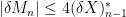${\vert\delta M_n\vert\le4(\delta X)^*_{n-1}}$ , Lemma 10 says that ${(M^*_\infty,[M]^{1/2}_\infty+4(\delta X)^*_\infty)}$ and ${([M]^{1/2}_\infty,M^*_\infty+4(\delta X)^*_\infty)}$ satisfy a good lambda inequality. So, by Lemma 5, for each ${0<p<\infty}$ there are positive constants ${C_{p,1},C_{p,2}}$ (independent of the choice of X) such that

$\displaystyle \setlength\arraycolsep{2pt} \begin{array}{rcl} &\displaystyle\Vert M^*_\infty\Vert_p&\displaystyle\le C_{p,1}\Vert [M]^{1/2}_\infty+4(\delta X)^*_\infty\Vert_p,\smallskip\\ &\displaystyle\Vert [M]^{1/2}_\infty\Vert_p&\displaystyle\le C_{p,2}\Vert M^*_\infty+4(\delta X)^*_\infty\Vert_p, \end{array}$

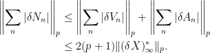
Now, as X=M+N, inequality (7) gives,

$\displaystyle \setlength\arraycolsep{2pt} \begin{array}{rl} \displaystyle\Vert X^*_\infty\Vert_p&\displaystyle\le\Vert M^*_\infty\Vert_p+2(p+1)\Vert(\delta X)^*_\infty\Vert_p\smallskip\\ &\displaystyle\le C_{p,1}\Vert[M]^{1/2}\Vert_p+2(p+1+2C_{p,1})\Vert(\delta X)^*_\infty\Vert_p. \end{array}$

Also, M=X–N so the triangle inequality together with (8) gives

$\displaystyle \Vert [M]^{1/2}_\infty\Vert\le\Vert[X]^{1/2}_\infty\Vert_p+2(p+1)\Vert(\delta X)^*_\infty\Vert_p.$

Hence,

$\displaystyle \Vert X^*_\infty\Vert_p\le C_{p,1}\Vert[X]^{1/2}\Vert_p+4(p+1+C_{p,1})\Vert(\delta X)^*_\infty\Vert_p$

and, as [X] is an increasing process with increments ${(\delta X_n)^2}$ , we have ${(\delta X)^*_\infty\le[X]^{1/2}_\infty}$ , giving the right hand inequality of (9) with ${C_p=C_{p,1}+4(p+1+C_{p,1})}$ .

A similar argument applies for the left hand side of (9). The triangle inequality ${\Vert[X]^{1/2}_\infty\Vert_p\le\Vert[M]^{1/2}_\infty\Vert_p+\Vert[N]^{1/2}_\infty\Vert_p}$ together with (8) gives,

$\displaystyle \setlength\arraycolsep{2pt} \begin{array}{rl} \displaystyle\Vert[X]^{1/2}_\infty\Vert_p &\displaystyle\le \Vert[M]^{1/2}_\infty\Vert_p+2(p+1)\Vert(\delta X)^*_\infty\Vert_p\smallskip\\ &\displaystyle\le C_{p,2}\Vert M^*_\infty\Vert_p+2(p+1+2C_{p,2})\Vert(\delta X)^*_\infty\Vert_p. \end{array}$

Then, as ${M^*\le X^*+N^*}$ , (7) gives,

$\displaystyle \Vert[X]^{1/2}_\infty\Vert_p\le C_{p,2}\Vert X^*_\infty\Vert_p+4(p+1+C_{p,2})\Vert(\delta X)^*_\infty\Vert_p.$

Finally, ${(\delta X)^*\le 2X^*}$ , so the left hand inequality of (9) is satisfied for ${c_p^{-1}=C_{p,2}+8(p+1+C_{p,2})}$ . ⬜

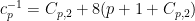Continuous-time Local Martingales

We finally prove the BDG inequality for ${p\ge 1}$ and an arbitrary continuous-time local martingale X, which will follow from applying a limiting argument to the discrete-time version stated in Theorem 11.

First, note that if ${\tau_n}$ is a sequence of stopping times increasing to infinity then ${X^*_{\tau_n},\ [X]^{1/2}_{\tau_n}}$ are monotonically increasing to ${X^*_\infty,\ [X]^{1/2}_\infty}$ . Then, by monotone convergence, it is enough to show that the BDG inequality is satisfied for the stopped processes ${X^{\tau_n}}$ .

As the quadratic variation has jumps ${\Delta[X]=(\Delta X)^2}$ , it follows that local ${L^p}$ -integrability of X is equivalent to local ${L^{p/2}}$ -integrability of [X] and, therefore, to local ${L^p}$ integrability of ${[X]^{1/2}}$ . If neither of ${X^*}$ and ${[X]^{1/2}}$ are locally ${L^p}$ -integrable then each term in (1) is infinite, so the inequality is trivially satisfied. We, therefore, suppose that one and, hence, both of ${X^*,[X]^{1/2}}$ are locally ${L^p}$ -integrable. By localization, we can suppose that ${X^*_\infty}$ and ${[X]^{1/2}_\infty}$ are both ${L^p}$ -integrable, in which case X is a proper martingale. 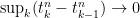Now, for each n, choose a sequence of times ${0=t^n_0\le t^n_1\le\cdots\uparrow\infty}$ such that ${\sup_k(t^n_k-t^n_{k-1})\rightarrow 0}$ as n goes to infinity. For example, ${t^n_k=k/n}$ . Then,

$\displaystyle [X]^{(n)}_t\equiv \sum_{k=1}^\infty (X_{t^n_k\wedge t}-X_{t^n_{k-1}\wedge t})^2$

converges ucp to [X]. Passing to a subsequence, if necessary, we suppose that ${[X]^{(n)}\rightarrow[X]}$ uniformly on compacts with probability one. So, ${M_t\equiv\sup_n[X]^{(n)}_t}$ will be a cadlag process with jumps

$\displaystyle \Delta M_t\le\sup_n\Delta[X]^{(n)}_t\le 2X^*_t\vert\Delta X_t\vert\le 4(X^*_\infty)^2,$

which are ${L^{p/2}}$ -bounded. So, by localization, we suppose that ${{\mathbb E}[M_\infty^{p/2}]}$ is finite. Fixing a time t and applying Theorem 11 to the discrete-time martingale ${\{X_{t^n_k\wedge t}\}_{k=0,1,\ldots}}$ gives

$\displaystyle c_p\left\Vert([X]^{(n)}_t)^{1/2}\right\Vert_p\le\left\Vert\sup_k\vert X_{t^n_k\wedge t}\vert\right\Vert_p\le C_p\left\Vert([X]^{(n)}_t)^{1/2}\right\Vert_p.$

Then, take the limit ${n\rightarrow\infty}$ followed by ${t\rightarrow\infty}$ and apply dominated convergence to ${([X]^{(n)}_t)^{p/2}\le M^{p/2}_\infty}$ and ${\max_k\vert X_{t^n_k\wedge t}\vert^p\le (X^*_\infty)^p}$ to get

$\displaystyle c_p\left\Vert[X]^{1/2}_\infty\right\Vert_p\le\left\Vert X^*_\infty\right\Vert_p\le C_p\left\Vert[X]^{1/2}_\infty\right\Vert_p.$

Raising to the p‘th power and replacing ${c_p^p,C_p^p}$ by ${c_p,C_p}$ gives the result.

Notes

Historically, the last case of the BDG inequalities to be proven was for p=1 in the paper `On the integrability of the martingale square function’ by Burgess Davis. It was here that the decomposition of the discrete-time martingale used above in the proof of Theorem 11 above was introduced. The proof given here follows, roughly, that given by Burkholder, Davis and Gundy in `Integral inequalities for convex functions of operators on martingales’. However, that paper considers a rather more general inequality, which I briefly mention now. A function ${F\colon{\mathbb R}_+\rightarrow{\mathbb R}_+}$ is said to be moderate if it is continuous, increasing and there are constants ${\alpha>1}$ and c such that ${F(\alpha x)\le c F(x)}$ . For example, if ${F(x)=x^p}$ then we can take ${c=\alpha^p}$ . Lemma 5 is easily generalized to show the existence of a constant C such that ${{\mathbb E}[F(X)]\le C{\mathbb E}[F(Y)]}$ for any pair of nonnegative random variables (X,Y) satisfying the good lambda inequality (3). Then, the proof for continuous local martingales above also shows that there are positive constants ${c_F,C_F}$ such that

$\displaystyle c_F{\mathbb E}\left[F\left([X]^{1/2}_\tau\right)\right]\le{\mathbb E}\left[F\left(X^*_\tau\right)\right]\le C_F{\mathbb E}\left[F\left([X]^{1/2}_\tau\right)\right]$

for any continuous local martingale X and stopping time ${\tau}$ . See here for a quick proof along the same lines. For arbitrary local martingales, it is necessary to impose the additional condition that F is convex, so that the required generalization of Lemma 8 holds. If ${F(x)=x^p}$ , this corresponds to ${p\ge 1}$ .

9 thoughts on “The Burkholder-Davis-Gundy Inequality”

soul says:

12 October 10 at 1:40 AM

this is quite useful for me!

pietro siorpaes says:

20 March 12 at 4:07 PM

I know that BDG inequalities hold also for local submartingales, which can be very useful sometimes.
Most likely the proof you gave would still work (with some equalities replaced by inequalities).
Could you please apply the few required changes and have the statement in this additional generality?
This would be useful as a reference, especially if you create a pdf version of the notes and post it on the Arxive…

P.S. Thank you for these wonderful notes!

Pingback: a nice optional sampling problem | Aquazorcarson's Blog
Dimbi says:

30 January 14 at 10:53 PM

Was this result published as a paper? just for reference

Eric says:

6 August 19 at 6:26 PM

In the last line of your proof of the good $\lambda$ inequality you subtract $\mathbb{E}[X^p]$ to complete the proof, but this only works if $\mathbb{E}[X^p]$ is finite. Is that an additional assumption in the theorem, or can you show that $\mathbb{E}[X^p] = \infty$ implies $\mathbb{E}[Y^p] = \infty$ under the assumptions?

1. George Lowther says:
  
  20 September 19 at 12:11 AM
  
  You are quite right, I missed this, but it is true that $\mathbb E[X^p]=\infty$ implies $\mathbb E[Y^p]=\infty$ . To see this, the good lambda inequality still holds if $\beta$ is replaced by $\beta\vee1$ and X is replaced by $X\wedge K$ (any positive K). Apply the result to this modified lambda inequality and let K go to infinity. I’ll update the proof when I have some time [Edit: it is now updated]. Thanks for pointing this out!
  
Helia Michaelson says:

7 October 19 at 5:09 PM

Could you please publish your references? Did you use any books for the proof? Thank you!

1. George Lowther says:
  
  10 October 19 at 12:08 AM
  
  As I mentioned in the post, the argument roughly follows `Integral inequalities for convex functions of operators on martingales’, http://projecteuclid.org/euclid.bsmsp/1200514221.
  
Hans says:

11 November 22 at 10:05 AM

The proof of Lemma 10 doesn’t seem to show that the quantities satisfy a good lambda inequality as the determined \psi does not vanish as \delta tends to 0, or did. I miss anything here?

	Tavin on Class (D) Processes
	George Lowther on Filtrations and Adapted P…
	faceet on Filtrations and Adapted P…
	George Lowther on Filtrations and Adapted P…
	facet on Filtrations and Adapted P…
	Zoltan on Class (D) Processes
	Zoltan on Class (D) Processes
	ARS on Stopping Times and the Debut…
	George Lowther on Upcrossings, Downcrossings, an…
	George Lowther on Stopping Times and the Debut…

The Burkholder-Davis-Gundy Inequality

Continuous Local Martingales

Discrete-time Martingales

Continuous-time Local Martingales

Notes

Published by George Lowther

9 thoughts on “The Burkholder-Davis-Gundy Inequality”

Leave a Reply Cancel reply

Continuous Local Martingales

Discrete-time Martingales

Continuous-time Local Martingales

Notes

Like this:

Related

Published by George Lowther

9 thoughts on “The Burkholder-Davis-Gundy Inequality”

Leave a Reply Cancel reply