Pathwise Burkholder-Davis-Gundy Inequalities

As covered earlier in my notes, the Burkholder-David-Gundy inequality relates the moments of the maximum of a local martingale M with its quadratic variation,

$\displaystyle c_p^{-1}{\mathbb E}[[M]^{p/2}_\tau]\le{\mathbb E}[\bar M_\tau^p]\le C_p{\mathbb E}[[M]^{p/2}_\tau].$

(1)

Here, ${\bar M_t\equiv\sup_{s\le t}\lvert M_s\rvert}$ is the running maximum, ${[M]}$ is the quadratic variation, ${\tau}$ is a stopping time, and the exponent ${p}$ is a real number greater than or equal to 1. Then, ${c_p}$ and ${C_p}$ are positive constants depending on p, but independent of the choice of local martingale and stopping time. Furthermore, for continuous local martingales, which are the focus of this post, the inequality holds for all ${p > 0}$ .

Since the quadratic variation used in my notes, by definition, starts at zero, the BDG inequality also required the local martingale to start at zero. This is not an important restriction, but it can be removed by requiring the quadratic variation to start at ${[M]_0=M_0^2}$ . Henceforth, I will assume that this is the case, which means that if we are working with the definition in my notes then we should add ${M_0^2}$ everywhere to the quadratic variation ${[M]}$ .

In keeping with the theme of the previous post on Doob’s inequalities, such martingale inequalities should have pathwise versions of the form

$\displaystyle c_p^{-1}[M]^{p/2}+\int\alpha dM\le\bar M^p\le C_p[M]^{p/2}+\int\beta dM$

(2)

for predictable processes ${\alpha,\beta}$ . Inequalities in this form are considerably stronger than (1), since they apply on all sample paths, not just on average. Also, we do not require M to be a local martingale — it is sufficient to be a (continuous) semimartingale. However, in the case where M is a local martingale, the pathwise version (2) does imply the BDG inequality (1), using the fact that stochastic integration preserves the local martingale property.

Lemma 1 Let X and Y be nonnegative increasing measurable processes satisfying ${X\le Y-N}$ for a local (sub)martingale N starting from zero. Then, ${{\mathbb E}[X_\tau]\le{\mathbb E}[Y_\tau]}$ for all stopping times ${\tau}$ .

Proof: Let ${\tau_n}$ be an increasing sequence of bounded stopping times increasing to infinity such that the stopped processes ${N^{\tau_n}}$ are submartingales. Then,

$\displaystyle {\mathbb E}[1_{\{\tau_n\ge\tau\}}X_\tau]\le{\mathbb E}[X_{\tau_n\wedge\tau}]={\mathbb E}[Y_{\tau_n\wedge\tau}]-{\mathbb E}[N_{\tau_n\wedge\tau}]\le{\mathbb E}[Y_{\tau_n\wedge\tau}]\le{\mathbb E}[Y_\tau].$

Letting n increase to infinity and using monotone convergence on the left hand side gives the result. ⬜

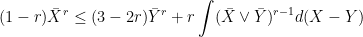
Moving on to the main statements of this post, I will mention that there are actually many different pathwise versions of the BDG inequalities. I opt for the especially simple statements given in Theorem 2 below. See the papers Pathwise Versions of the Burkholder-Davis Gundy Inequality by Bieglböck and Siorpaes, and Applications of Pathwise Burkholder-Davis-Gundy inequalities by Soirpaes, for slightly different approaches, although these papers do also effectively contain proofs of (3,4) for the special case of ${r=1/2}$ . As usual, I am using ${x\vee y}$ to represent the maximum of two numbers.

Theorem 2 Let X and Y be nonnegative continuous processes with ${X_0=Y_0}$ . For any ${0 < r\le1}$ we have,

$\displaystyle (1-r)\bar X^r\le (3-2r)\bar Y^r+r\int(\bar X\vee\bar Y)^{r-1}d(X-Y)$ (3)

and, if X is increasing, this can be improved to,

$\displaystyle \bar X^r\le (2-r)\bar Y^r+r\int(\bar X\vee\bar Y)^{r-1}d(X-Y).$ (4)

If ${r\ge1}$ and X is increasing then,

$\displaystyle \bar X^r\le r^{r\vee 2}\,\bar Y^r+r^2\int(\bar X\vee\bar Y)^{r-1}d(X-Y).$ (5)

Continue reading “Pathwise Burkholder-Davis-Gundy Inequalities” →

Girsanov Transformations

Girsanov transformations describe how Brownian motion and, more generally, local martingales behave under changes of the underlying probability measure. Let us start with a much simpler identity applying to normal random variables. Suppose that X and ${Y=(Y^1,\ldots,Y^n)}$ are jointly normal random variables defined on a probability space ${(\Omega,\mathcal{F},{\mathbb P})}$ . Then ${U\equiv\exp(X-\frac{1}{2}{\rm Var}(X)-{\mathbb E}[X])}$ is a positive random variable with expectation 1, and a new measure ${{\mathbb Q}=U\cdot{\mathbb P}}$ can be defined by ${{\mathbb Q}(A)={\mathbb E}[1_AU]}$ for all sets ${A\in\mathcal{F}}$ . Writing ${{\mathbb E}_{\mathbb Q}}$ for expectation under the new measure, then ${{\mathbb E}_{\mathbb Q}[Z]={\mathbb E}[UZ]}$ for all bounded random variables Z. The expectation of a bounded measurable function ${f\colon{\mathbb R}^n\rightarrow{\mathbb R}}$ of Y under the new measure is

$\displaystyle {\mathbb E}_{\mathbb Q}\left[f(Y)\right]={\mathbb E}\left[f\left(Y+{\rm Cov}(X,Y)\right)\right],$

(1)

where ${{\rm Cov}(X,Y)}$ is the covariance. This is a vector whose i’th component is the covariance ${{\rm Cov}(X,Y^i)}$ . So, Y has the same distribution under ${{\mathbb Q}}$ as ${Y+{\rm Cov}(X,Y)}$ has under ${{\mathbb P}}$ . That is, when changing to the new measure, Y remains jointly normal with the same covariance matrix, but its mean increases by ${{\rm Cov}(X,Y)}$ . Equation (1) follows from a straightforward calculation of the characteristic function of Y with respect to both ${{\mathbb P}}$ and ${{\mathbb Q}}$ .

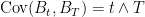Now consider a standard Brownian motion B and fix a time ${T>0}$ and a constant ${\mu}$ . Then, for all times ${t\ge 0}$ , the covariance of ${B_t}$ and ${B_T}$ is ${{\rm Cov}(B_t,B_T)=t\wedge T}$ . Applying (1) to the measure ${{\mathbb Q}=\exp(\mu B_T-\mu^2T/2)\cdot{\mathbb P}}$ shows that

$\displaystyle B_t=\tilde B_t + \mu (t\wedge T)$

where ${\tilde B}$ is a standard Brownian motion under ${{\mathbb Q}}$ . Under the new measure, B has gained a constant drift of ${\mu}$ over the interval ${[0,T]}$ . Such transformations are widely applied in finance. For example, in the Black-Scholes model of option pricing it is common to work under a risk-neutral measure, which transforms the drift of a financial asset to be the risk-free rate of return. Girsanov transformations extend this idea to much more general changes of measure, and to arbitrary local martingales. However, as shown below, the strongest results are obtained for Brownian motion which, under a change of measure, just gains a stochastic drift term. Continue reading “Girsanov Transformations” →

Time-Changed Brownian Motion

From the definition of standard Brownian motion B, given any positive constant c, ${B_{ct}-B_{cs}}$ will be normal with mean zero and variance c(t–s) for times ${t>s\ge 0}$ . So, scaling the time axis of Brownian motion B to get the new process ${B_{ct}}$ just results in another Brownian motion scaled by the factor ${\sqrt{c}}$ .

This idea is easily generalized. Consider a measurable function ${\xi\colon{\mathbb R}_+\rightarrow{\mathbb R}_+}$ and Brownian motion B on the filtered probability space ${(\Omega,\mathcal{F},\{\mathcal{F}_t\}_{t\ge 0},{\mathbb P})}$ . So, ${\xi}$ is a deterministic process, not depending on the underlying probability space ${\Omega}$ . If ${\theta(t)\equiv\int_0^t\xi^2_s\,ds}$ is finite for each ${t>0}$ then the stochastic integral ${X=\int\xi\,dB}$ exists. Furthermore, X will be a Gaussian process with independent increments. For piecewise constant integrands, this results from the fact that linear combinations of joint normal variables are themselves normal. The case for arbitrary deterministic integrands follows by taking limits. Also, the Ito isometry says that ${X_t-X_s}$ has variance

$\displaystyle \setlength\arraycolsep{2pt} \begin{array}{rl} \displaystyle{\mathbb E}\left[\left(\int_s^t\xi\,dB\right)^2\right]&\displaystyle={\mathbb E}\left[\int_s^t\xi^2_u\,du\right]\smallskip\\ &\displaystyle=\theta(t)-\theta(s)\smallskip\\ &\displaystyle={\mathbb E}\left[(B_{\theta(t)}-B_{\theta(s)})^2\right]. \end{array}$

So, ${\int\xi\,dB=\int\sqrt{\theta^\prime(t)}\,dB_t}$ has the same distribution as the time-changed Brownian motion ${B_{\theta(t)}}$ .

With the help of Lévy’s characterization, these ideas can be extended to more general, non-deterministic, integrands and to stochastic time-changes. In fact, doing this leads to the startling result that all continuous local martingales are just time-changed Brownian motion. Continue reading “Time-Changed Brownian Motion” →

Lévy’s Characterization of Brownian Motion

Standard Brownian motion, ${\{B_t\}_{t\ge 0}}$ , is defined to be a real-valued process satisfying the following properties.

${B_0=0}$ .
${B_t-B_s}$ is normally distributed with mean 0 and variance t–s independently of ${\{B_u\colon u\le s\}}$ , for any ${t>s\ge 0}$ .
B has continuous sample paths.

As always, it only really matters is that these properties hold almost surely. Now, to apply the techniques of stochastic calculus, it is assumed that there is an underlying filtered probability space ${(\Omega,\mathcal{F},\{\mathcal{F}_t\}_{t\ge 0},{\mathbb P})}$ , which necessitates a further definition; a process B is a Brownian motion on a filtered probability space ${(\Omega,\mathcal{F},\{\mathcal{F}_t\}_{t\ge 0},{\mathbb P})}$ if in addition to the above properties it is also adapted, so that ${B_t}$ is ${\mathcal{F}_t}$ -measurable, and ${B_t-B_s}$ is independent of ${\mathcal{F}_s}$ for each ${t>s\ge 0}$ . Note that the above condition that ${B_t-B_s}$ is independent of ${\{B_u\colon u\le s\}}$ is not explicitly required, as it also follows from the independence from ${\mathcal{F}_s}$ . According to these definitions, a process is a Brownian motion if and only if it is a Brownian motion with respect to its natural filtration.

The property that ${B_t-B_s}$ has zero mean independently of ${\mathcal{F}_s}$ means that Brownian motion is a martingale. Furthermore, we previously calculated its quadratic variation as ${[B]_t=t}$ . An incredibly useful result is that the converse statement holds. That is, Brownian motion is the only local martingale with this quadratic variation. This is known as Lévy’s characterization, and shows that Brownian motion is a particularly general stochastic process, justifying its ubiquitous influence on the study of continuous-time stochastic processes.

Theorem 1 (Lévy’s Characterization of Brownian Motion) Let X be a local martingale with ${X_0=0}$ . Then, the following are equivalent.

X is standard Brownian motion on the underlying filtered probability space.

X is continuous and ${X^2_t-t}$ is a local martingale.

X has quadratic variation ${[X]_t=t}$ .

Continue reading “Lévy’s Characterization of Brownian Motion” →

The Burkholder-Davis-Gundy Inequality

The Burkholder-Davis-Gundy inequality is a remarkable result relating the maximum of a local martingale with its quadratic variation. Recall that [X] denotes the quadratic variation of a process X, and ${X^*_t\equiv\sup_{s\le t}\vert X_s\vert}$ is its maximum process.

Theorem 1 (Burkholder-Davis-Gundy) For any ${1\le p<\infty}$ there exist positive constants ${c_p,C_p}$ such that, for all local martingales X with ${X_0=0}$ and stopping times ${\tau}$ , the following inequality holds.

$\displaystyle c_p{\mathbb E}\left[ [X]^{p/2}_\tau\right]\le{\mathbb E}\left[(X^*_\tau)^p\right]\le C_p{\mathbb E}\left[ [X]^{p/2}_\tau\right].$ (1)

Furthermore, for continuous local martingales, this statement holds for all ${0<p<\infty}$ .

A proof of this result is given below. For ${p\ge 1}$ , the theorem can also be stated as follows. The set of all cadlag martingales X starting from zero for which ${{\mathbb E}[(X^*_\infty)^p]}$ is finite is a vector space, and the BDG inequality states that the norms ${X\mapsto\Vert X^*_\infty\Vert_p={\mathbb E}[(X^*_\infty)^p]^{1/p}}$ and ${X\mapsto\Vert[X]^{1/2}_\infty\Vert_p}$ are equivalent.

The special case p=2 is the easiest to handle, and we have previously seen that the BDG inequality does indeed hold in this case with constants ${c_2=1}$ , ${C_2=4}$ . The significance of Theorem 1, then, is that this extends to all ${p\ge1}$ .

One reason why the BDG inequality is useful in the theory of stochastic integration is as follows. Whereas the behaviour of the maximum of a stochastic integral is difficult to describe, the quadratic variation satisfies the simple identity ${\left[\int\xi\,dX\right]=\int\xi^2\,d[X]}$ . Recall, also, that stochastic integration preserves the local martingale property. Stochastic integration does not preserve the martingale property. In general, integration with respect to a martingale only results in a local martingale, even for bounded integrands. In many cases, however, stochastic integrals are indeed proper martingales. The Ito isometry shows that this is true for square integrable martingales, and the BDG inequality allows us to extend the result to all ${L^p}$ -integrable martingales, for ${p> 1}$ .

Theorem 2 Let X be a cadlag ${L^p}$ -integrable martingale for some ${1<p<\infty}$ , so that ${{\mathbb E}[\vert X_t\vert^p]<\infty}$ for each t. Then, for any bounded predictable process ${\xi}$ , ${Y\equiv\int\xi\,dX}$ is also an ${L^p}$ -integrable martingale.

Continue reading “The Burkholder-Davis-Gundy Inequality” →

Continuous Local Martingales

Continuous local martingales are a particularly well behaved subset of the class of all local martingales, and the results of the previous two posts become much simpler in this case. First, the continuous local martingale property is always preserved by stochastic integration.

Theorem 1 If X is a continuous local martingale and ${\xi}$ is X-integrable, then ${\int\xi\,dX}$ is a continuous local martingale.

Proof: As X is continuous, ${Y\equiv\int\xi\,dX}$ will also be continuous and, therefore, locally bounded. Then, by preservation of the local martingale property, Y is a local martingale. ⬜

Next, the quadratic variation of a continuous local martingale X provides us with a necessary and sufficient condition for X-integrability.

Theorem 2 Let X be a continuous local martingale. Then, a predictable process ${\xi}$ is X-integrable if and only if

$\displaystyle \int_0^t\xi^2\,d[X]<\infty$

for all ${t>0}$ .

Continue reading “Continuous Local Martingales” →

Quadratic Variations and the Ito Isometry

As local martingales are semimartingales, they have a well-defined quadratic variation. These satisfy several useful and well known properties, such as the Ito isometry, which are the subject of this post. First, the covariation [X,Y] allows the product XY of local martingales to be decomposed into local martingale and FV terms. Consider, for example, a standard Brownian motion B. This has quadratic variation ${[B]_t=t}$ and it is easily checked that ${B^2_t-t}$ is a martingale.

Lemma 1 If X and Y are local martingales then XY-[X,Y] is a local martingale.

In particular, ${X^2-[X]}$ is a local martingale for all local martingales X.

Proof: Integration by parts gives

$\displaystyle XY-[X,Y] = X_0Y_0+\int X_-\,dY+\int Y_-\,dX$

which, by preservation of the local martingale property, is a local martingale. ⬜

Continue reading “Quadratic Variations and the Ito Isometry” →

The Generalized Ito Formula

Recall that Ito’s lemma expresses a twice differentiable function ${f}$ applied to a continuous semimartingale ${X}$ in terms of stochastic integrals, according to the following formula

$\displaystyle f(X) = f(X_0)+\int f^\prime(X)\,dX + \frac{1}{2}\int f^{\prime\prime}(X)\,d[X].$

(1)

In this form, the result only applies to continuous processes but, as I will show in this post, it is possible to generalize to arbitrary noncontinuous semimartingales. The result is also referred to as Ito’s lemma or, to distinguish it from the special case for continuous processes, it is known as the generalized Ito formula or generalized Ito’s lemma.

If equation (1) is to be extended to noncontinuous processes then, there are two immediate points to be considered. The first is that if the process ${X}$ is not continuous then it need not be a predictable process, so ${f^\prime(X),f^{\prime\prime}(X)}$ need not be predictable either. So, the integrands in (1) will not be ${X}$ -integrable. To remedy this, we should instead use the left limits ${X_{t-}}$ in the integrands, which is left-continuous and adapted and therefore is predictable. The second point is that the jumps of the left hand side of (1) are equal to ${\Delta f(X)}$ and, on the right, they are ${f^\prime(X_-)\Delta X+\frac{1}{2}f^{\prime\prime}(X_-)\Delta X^2}$ . There is no reason that these should be equal, and (1) cannot possibly hold in general. To fix this, we can simply add on the correction to the jump terms on the right hand side,

$\displaystyle \setlength\arraycolsep{2pt} \begin{array}{rl} \displaystyle f(X_t) =&\displaystyle f(X_0)+\int_0^t f^\prime(X_-)\,dX + \frac{1}{2}\int_0^t f^{\prime\prime}(X_-)\,d[X]\smallskip\\ &\displaystyle +\sum_{s\le t}\left(\Delta f(X_s)-f^\prime(X_{s-})\Delta X_s-\frac{1}{2}f^{\prime\prime}(X_{s-})\Delta X_s^2\right). \end{array}$

(2)

Continue reading “The Generalized Ito Formula” →

Ito’s Lemma

Ito’s lemma, otherwise known as the Ito formula, expresses functions of stochastic processes in terms of stochastic integrals. In standard calculus, the differential of the composition of functions ${f(x), x(t)}$ satisfies ${df(x(t))=f^\prime(x(t))dx(t)}$ . This is just the chain rule for differentiation or, in integral form, it becomes the change of variables formula.

In stochastic calculus, Ito’s lemma should be used instead. For a twice differentiable function ${f}$ applied to a continuous semimartingale ${X}$ , it states the following,

$\displaystyle df(X) = f^\prime(X)\,dX + \frac{1}{2}f^{\prime\prime}(X)\,dX^2.$

This can be understood as a Taylor expansion up to second order in ${dX}$ , where the quadratic term ${dX^2\equiv d[X]}$ is the quadratic variation of the process ${X}$ .

A d-dimensional process ${X=(X^1,\ldots,X^d)}$ is said to be a semimartingale if each of its components, ${X^i}$ , are semimartingales. The first and second order partial derivatives of a function are denoted by ${D_if}$ and ${D_{ij}f}$ , and I make use of the summation convention where indices ${i,j}$ which occur twice in a single term are summed over. Then, the statement of Ito’s lemma is as follows.

Theorem 1 (Ito’s Lemma) Let ${X=(X^1,\ldots,X^d)}$ be a continuous d-dimensional semimartingale taking values in an open subset ${U\subseteq{\mathbb R}^d}$ . Then, for any twice continuously differentiable function ${f\colon U\rightarrow{\mathbb R}}$ , ${f(X)}$ is a semimartingale and,

$\displaystyle df(X) = D_if(X)\,dX^i + \frac{1}{2}D_{ij}f(X)\,d[X^i,X^j].$ (1)

Continue reading “Ito’s Lemma” →

Properties of Quadratic Variations

Being able to handle quadratic variations and covariations of processes is very important in stochastic calculus. Apart from appearing in the integration by parts formula, they are required for the stochastic change of variables formula, known as Ito’s lemma, which will be the subject of the next post. Quadratic covariations satisfy several simple relations which make them easy to handle, especially in conjunction with the stochastic integral.

Recall from the previous post that the covariation ${[X,Y]}$ is a cadlag adapted process, so that its jumps ${\Delta [X,Y]_t\equiv [X,Y]_t-[X,Y]_{t-}}$ are well defined.

Lemma 1 If ${X,Y}$ are semimartingales then

$\displaystyle \Delta [X,Y]=\Delta X\Delta Y.$ (1)

In particular, ${\Delta [X]=\Delta X^2}$ .

Proof: Taking the jumps of the integration by parts formula for ${XY}$ gives

$\displaystyle \Delta XY = X_{-}\Delta Y + Y_{-}\Delta X + \Delta [X,Y],$

and rearranging this gives the result. ⬜

An immediate consequence is that quadratic variations and covariations involving continuous processes are continuous. Another consequence is that the sum of the squares of the jumps of a semimartingale over any bounded interval must be finite.

Corollary 2 Every semimartingale ${X}$ satisfies

$\displaystyle \sum_{s\le t}\Delta X^2_s\le [X]_t<\infty.$

Proof: As ${[X]}$ is increasing, the inequality ${[X]_t\ge \sum_{s\le t}\Delta [X]_s}$ holds. Substituting in ${\Delta[X]=\Delta X^2}$ gives the result. ⬜

Next, the following result shows that covariations involving continuous finite variation processes are zero. As Lebesgue-Stieltjes integration is only defined for finite variation processes, this shows why quadratic variations do not play an important role in standard calculus. For noncontinuous finite variation processes, the covariation must have jumps satisfying (1), so will generally be nonzero. In this case, the covariation is just given by the sum over these jumps. Integration with respect to any FV process ${V}$ can be defined as the Lebesgue-Stieltjes integral on the sample paths, which is well defined for locally bounded measurable integrands and, when the integrand is predictable, agrees with the stochastic integral.

Lemma 3 Let ${X}$ be a semimartingale and ${V}$ be an FV process. Their covariation is

$\displaystyle [X,V]_t = \int_0^t \Delta X\,dV = \sum_{s\le t}\Delta X_s\Delta V_s.$ (2)

In particular, if either of ${X}$ or ${V}$ is continuous then ${[X,V]=0}$ .

Continue reading “Properties of Quadratic Variations” →

	Harry on Filtrations and Adapted P…
	Anonymous on Analytic Sets
	Daniel on Analytic Sets
	Sid on Martingale Convergence
	northwiz on Preservation of the Local Mart…
	George Lowther on Martingale Convergence
	Sid on Martingale Convergence
	George Lowther on The Burkholder-Davis-Gundy Ine…
	George Lowther on Preservation of the Local Mart…
	northwiz on Preservation of the Local Mart…

Like this:

Like this:

Like this:

Like this:

Like this:

Like this:

Like this:

Like this:

Like this:

Like this: