Recall Doob’s inequalities, covered earlier in these notes, which bound expectations of functions of the maximum of a martingale in terms of its terminal distribution. Although these are often applied to martingales, they hold true more generally for cadlag submartingales. Here, I use  to denote the running maximum of a process.
Theorem 1 Let X be a nonnegative cadlag submartingale. Then,
In particular, for a cadlag martingale X, then  is a submartingale, so theorem 1 applies with in place of X.
We also saw the following much stronger (sub)martingale inequality in the post on the maximum maximum of martingales with known terminal distribution.
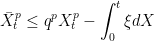
Theorem 2 Let X be a cadlag submartingale. Then, for any real K and nonnegative real t,
![\displaystyle {\mathbb P}(\bar X_t\ge K)\le\inf_{x < K}\frac{{\mathbb E}[(X_t-x)_+]}{K-x}.](https://s0.wp.com/latex.php?latex=%5Cdisplaystyle++%7B%5Cmathbb+P%7D%28%5Cbar+X_t%5Cge+K%29%5Cle%5Cinf_%7Bx+%3C+K%7D%5Cfrac%7B%7B%5Cmathbb+E%7D%5B%28X_t-x%29_%2B%5D%7D%7BK-x%7D.+&bg=ffffff&fg=000000&s=0&c=20201002) |
(1) |
This is particularly sharp, in the sense that for any distribution for  , there exists a martingale with this terminal distribution for which (1) becomes an equality simultaneously for all values of K. Furthermore, all of the inequalities stated in theorem 1 follow from (1). For example, the first one is obtained by taking
  in (1). The remaining two can also be proved from (1) by integrating over K.
Note that all of the submartingale inequalities above are of the form
![\displaystyle {\mathbb E}[F(\bar X_t)]\le{\mathbb E}[G(X_t)]](https://s0.wp.com/latex.php?latex=%5Cdisplaystyle++%7B%5Cmathbb+E%7D%5BF%28%5Cbar+X_t%29%5D%5Cle%7B%5Cmathbb+E%7D%5BG%28X_t%29%5D+&bg=ffffff&fg=000000&s=0&c=20201002) |
(2) |
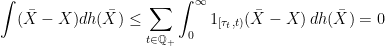
for certain choices of functions  . The aim of this post is to show how they have a more general `pathwise’ form,
 |
(3) |
for some nonnegative predictable process  . It is relatively straightforward to show that (2) follows from (3) by noting that the integral is a submartingale and, hence, has nonnegative expectation. To be rigorous, there are some integrability considerations to deal with, so a proof will be included later in this post.
Inequality (3) is required to hold almost everywhere, and not just in expectation, so is a considerably stronger statement than the standard martingale inequalities. Furthermore, it is not necessary for X to be a submartingale for (3) to make sense, as it holds for all semimartingales. We can go further, and even drop the requirement that X is a semimartingale. As we will see, in the examples covered in this post,  will be of the form
  for an increasing right-continuous function
  , so integration by parts can be used,
 |
(4) |
The right hand side of (4) is well-defined for any cadlag real-valued process, by using the pathwise Lebesgue–Stieltjes integral with respect to the increasing process  , so can be used as the definition of
  . In the case where X is a semimartingale, integration by parts ensures that this agrees with the stochastic integral
  . Since we now have an interpretation of (3) in a pathwise sense for all cadlag processes X, it is no longer required to suppose that X is a submartingale, a semimartingale, or even require the existence of an underlying probability space. All that is necessary is for
  to be a cadlag real-valued function. Hence, we reduce the martingale inequalities to straightforward results of real-analysis not requiring any probability theory and, consequently, are much more general. I state the precise pathwise generalizations of Doob’s inequalities now, leaving the proof until later in the post. As the first of inequality of theorem 1 is just the special case of (1) with , we do not need to explicitly include this here.
Theorem 3 Let X be a cadlag process and t be a nonnegative time.
- For real
 ,
,
 |
(5) |
where  .
.
- If X is nonnegative and p,q are positive reals with
 then,
then,
 |
(6) |
where  .
.
- If X is nonnegative then,
 |
(7) |
where 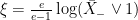 .
.
The pathwise inequalities can be stated quite succinctly in discrete time, in which case they become simple inequalities for finite sequences of real numbers. Given any such sequence  , set
, set  . By considering the cadlag process
  over
over  , the inequalities stated in theorem 3 are of the form,
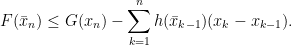 |
(8) |
The more general continuous-time inequalities can also be derived as a limit of the discrete-time case, so this is still quite general. Furthermore, if  is a discrete-time submartingale, then taking expectations of (8) gives the discrete version of Doob’s inequalities, from which the continuous-time versions can be obtained by taking limits. Alternatively, we can show directly that Doob’s inequalities follow from the pathwise versions by taking expectations in continuous time.
Lemma 4 Let X be a cadlag submartingale taking values in an interval  and satisfying (3) for some
  , where G is convex and increasing, and for some nonnegative and locally bounded predictable process . Then,
![\displaystyle {\mathbb E}[F(\bar X_\tau)]\le{\mathbb E}[G(X_\tau)]](https://s0.wp.com/latex.php?latex=%5Cdisplaystyle++%7B%5Cmathbb+E%7D%5BF%28%5Cbar+X_%5Ctau%29%5D%5Cle%7B%5Cmathbb+E%7D%5BG%28X_%5Ctau%29%5D+&bg=ffffff&fg=000000&s=0&c=20201002)
for all bounded stopping times  .
.
Proof: As is locally bounded and nonnegative,  is locally a submartingale and, hence, there exists a sequence of stopping times
  increasing to infinity such that
  are submartingales. Therefore,
 ![{{\mathbb E}[M_{\tau_n\wedge\tau}]\ge0}](https://s0.wp.com/latex.php?latex=%7B%7B%5Cmathbb+E%7D%5BM_%7B%5Ctau_n%5Cwedge%5Ctau%7D%5D%5Cge0%7D&bg=ffffff&fg=000000&s=0&c=20201002) . Next, as G is convex and increasing,
. Next, as G is convex and increasing,  is a submartingale. So, taking expectations of (3) at time
  ,
,
![\displaystyle {\mathbb E}[1_{\{\tau_n\ge\tau\}}F(\bar X_\tau)]\le{\mathbb E}[F(\bar X_{\tau\wedge\tau_n})]\le{\mathbb E}[G(X_{\tau\wedge\tau_n})]\le{\mathbb E}[G(X_\tau)].](https://s0.wp.com/latex.php?latex=%5Cdisplaystyle++%7B%5Cmathbb+E%7D%5B1_%7B%5C%7B%5Ctau_n%5Cge%5Ctau%5C%7D%7DF%28%5Cbar+X_%5Ctau%29%5D%5Cle%7B%5Cmathbb+E%7D%5BF%28%5Cbar+X_%7B%5Ctau%5Cwedge%5Ctau_n%7D%29%5D%5Cle%7B%5Cmathbb+E%7D%5BG%28X_%7B%5Ctau%5Cwedge%5Ctau_n%7D%29%5D%5Cle%7B%5Cmathbb+E%7D%5BG%28X_%5Ctau%29%5D.+&bg=ffffff&fg=000000&s=0&c=20201002)
Letting n increase to infinity and applying monotone convergence on the left hand side gives the result. ⬜
See Gushchin, On pathwise counterparts of Doob’s maximal inequalities, and the references contained therein, for more information on the pathwise approach.
To prove the pathwise inequalities, I start with the following simple, but very neat, identity. This actually extends to all measurable and locally bounded functions h in the case where X is a semimartingale (applying the monotone class theorem). However, I state it only for the required situation where  is right-continuous and increasing, in which case the integral makes sense for all cadlag processes X.
Lemma 5 Let X be a cadlag process and be increasing and right-continuous. Then,
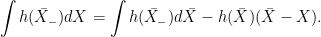 |
(9) |
Proof: Applying (4),

So, to prove (9) it only needs to be shown that

and, as is an increasing process, this integral is understood in the pathwise Lebesgue-Stieltjes sense.
For any  let
let  be the last time before t at which
  ,
,

Then,  is constant on
  and, hence,

As  , we see that
  whenever
  and, hence, the above equality is identically zero. Next, if s is any time at which
  then, by right-continuity,
  for all
  sufficiently close to s, giving
  . Hence, using the fact that the positive rationals
  are dense in
  , by countable additivity,
as required. ⬜
We obtain the following consequence of lemma 9. I am using  to denote the right-hand derivative which, as
  is convex, is right-continuous and increasing.
Corollary 6 Let X be a cadlag process and  be convex with
  . Then,
 |
(10) |
Proof: By (9) it is sufficient to show that  . See, for example, lemma 1 of the post on local times. Alternatively, by approximating by continuous functions, we can suppose that it is continuous (and increasing). So, by convexity,

Hence, for any sequence of times  ,
,

Letting the mesh  go to zero, bounded convergence shows that the right hand side of the above inequality tends to
  , giving the result. ⬜
I did not include terms involving the starting value  in the pathwise inequalities, just in order to have very simple statements. However, they can be included if desired, in which case we should subtract
  from the right hand side of (10) and, the proof given still holds. In fact, if we do this, then (10) is very sharp, and is an equality whenever
  is continuous. I finally give proofs of the pathwise inequalities, as an application of corollary 6.
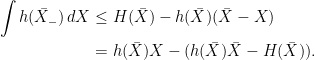
Proof of Theorem 3: Applying (10) with  and
and 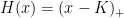 gives,
Dividing through by  gives (5).
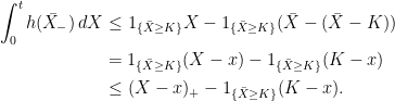
Next, apply (10) with  and
and  ,
,

using the AM-GM inequality. This gives (6) as required.
Finally, apply (10) with 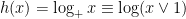 and
and  ,
,
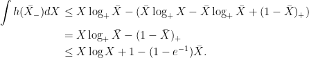
The last inequality is using (2) of the original post on martingale inequalities, and we obtain (7). ⬜

for all
.
for all
.
.
