The Maximum Maximum of Martingales with Known Terminal Distribution

In this post I will be concerned with the following problem — given a martingale X for which we know the distribution at a fixed time, and we are given nothing else, what is the best bound we can obtain for the maximum of X up until that time? This is a question with a long history, starting with Doob’s inequalities which bound the maximum in the ${L^p}$ norms and in probability. Later, Blackwell and Dubins (3), Dubins and Gilat (5) and Azema and Yor (1,2) showed that the maximum is bounded above, in stochastic order, by the Hardy-Littlewood transform of the terminal distribution. Furthermore, this bound is the best possible in the sense that there do exists martingales for which it can be attained, for any permissible terminal distribution. Hobson (7,8) considered the case where the starting law is also known, and this was further generalized to the case with a specified distribution at an intermediate time by Brown, Hobson and Rogers (4). Finally, Henry-Labordère, Obłój, Spoida and Touzi (6) considered the case where the distribution of the martingale is specified at an arbitrary set of times. In this post, I will look at the case where only the terminal distribution is specified. This leads to interesting constructions of martingales and, in particular, of continuous martingales with specified terminal distributions, with close connections to the Skorokhod embedding problem.

I will be concerned with the maximum process of a cadlag martingale X,

$\displaystyle X^*_t=\sup_{s\le t}X_s,$

which is increasing and adapted. We can state and prove the bound on ${X^*}$ relatively easily, although showing that it is optimal is more difficult. As the result holds more generally for submartingales, I state it in this case, although I am more concerned with martingales here.

Theorem 1 If X is a cadlag submartingale then, for each ${t\ge0}$ and ${x\in{\mathbb R}}$ ,

$\displaystyle {\mathbb P}\left(X^*_t\ge x\right)\le\inf_{y < x}\frac{{\mathbb E}\left[(X_t-y)_+\right]}{x-y}.$ (1)

Proof: We just need to show that the inequality holds for each ${y < x}$ , and then it immediately follows for the infimum. Choosing ${y < x^\prime < x}$ , consider the stopping time

$\displaystyle \tau=\inf\{s\ge0\colon X_s\ge x^\prime\}.$

Then, ${\tau \le t}$ and ${X_\tau\ge x^\prime}$ whenever ${X^*_t \ge x}$ . As ${f(z)\equiv(z-y)_+}$ is nonnegative and increasing in z, this means that ${1_{\{X^*_t\ge x\}}}$ is bounded above by ${f(X_{\tau\wedge t})/f(x^\prime)}$ . Taking expectations,

$\displaystyle {\mathbb P}\left(X^*_t\ge x\right)\le{\mathbb E}\left[f(X_{\tau\wedge t})\right]/f(x^\prime).$

Since f is convex and increasing, ${f(X)}$ is a submartingale so, using optional sampling,

$\displaystyle {\mathbb P}\left(X^*_t\ge x\right)\le{\mathbb E}\left[f(X_t)\right]/f(x^\prime).$

Letting ${x^\prime}$ increase to ${x}$ gives the result. ⬜

The bound stated in Theorem 1 is also optimal, and can be achieved by a continuous martingale. In this post, all measures on ${{\mathbb R}}$ are defined with respect to the Borel sigma-algebra.

Theorem 2 If ${\mu}$ is a probability measure on ${{\mathbb R}}$ with ${\int\lvert x\rvert\,d\mu(x) < \infty}$ and ${t > 0}$ then there exists a continuous martingale X (defined on some filtered probability space) such that ${X_t}$ has distribution ${\mu}$ and (1) is an equality for all ${x\in{\mathbb R}}$ .

I will not prove this yet, as the construction of martingales verifying this result will be given further below. The proof of Theorem 1 given above should, however, give a good clue as to how the optimal bound can be attained. In order for the (submartingale) inequality used to actually be an equality, it is required that the process ${(X_t-y)_+}$ be a martingale starting from the time ${\tau}$ , and to be equal to 0 at time t if the level x is not reached. This is the case if, for some ${y < x}$ , we have ${X_t\ge y}$ whenever ${X^*_t\ge x}$ and ${X_t\le y}$ whenever ${X^*_t < x}$ . Martingales constructed with this property will be given below.

Theorem 2 is particularly strong, as not only does it imply that the bound (1) is optimal, but also that there exists a single continuous martingale making (1) an equality simultaneously for all values of x. A consequence of this is that we also achieve an optimal upper bound for ${{\mathbb E}[f(X^*_t)]}$ for all bounded increasing functions ${f}$ . This is maybe best understood in terms of the stochastic order on measures, denoted by ${\preceq}$ . We write ${\mu\preceq\nu}$ for probability measures ${\mu,\nu}$ on ${{\mathbb R}}$ if either of the following equivalent conditions are satisfied.

${\mu([x,\infty))\le\nu([x,\infty))}$ for all real x.
${\mu(f)\le\nu(f)}$ for all bounded increasing ${f}$ .
${\mu(f)\le\nu(f)}$ for all nonnegative increasing ${f}$ .
there exists some probability space with real random variables ${X,Y}$ with laws ${\mu,\nu}$ respectively such that ${X\le Y}$ (a.s.).

The equivalence of these conditions is straightforward, with only the existence of the random variables X,Y in the final statement needing further explanation. If ${F(x)=\mu([x,\infty))}$ , ${G(x)=\nu([x,\infty))}$ then, for any uniform random variable U on the unit interval, ${X=F^{-1}(U)}$ and ${Y=G^{-1}(U)}$ will have laws ${\mu,\nu}$ respectively, and satisfy ${X\le Y}$ .

Next, the Hardy-Littlewood transform of a measure ${\mu}$ with ${\int\lvert x\rvert\,d\mu(x) < \infty}$ is defined by

$\displaystyle \mu^*\left([x,\infty)\right)=\inf_{y < x}(x-y)^{-1}\int_x^\infty(z-y)\,d\mu(z).$

(2)

It can be seen that this is left-continuous and decreasing from 1 to 0 as x increases from ${-\infty}$ to ${+\infty}$ , so gives a well-defined Borel measure ${\mu^*}$ . As will be seen below in Lemma 6, the Hardy-Littlewood transform can alternatively be defined as follows. If ${h(U)}$ has law ${\mu}$ , for a decreasing integrable function h and uniform random variable U on ${[0,1]}$ , then ${\bar h(U)}$ has law ${\mu^*}$ where ${\bar h}$ is the running average of h. Next, I denote the law of a real random variable V by ${\mu_V}$ .

One construction of a martingale with terminal distribution ${\mu}$ is given simply by setting ${X_s=m\equiv\int x\,d\mu(x)}$ for all ${s < t}$ , in which case ${X^*_t\ge m}$ . This means that the probability in (1) must be 1 for all ${x\le m}$ . Correspondingly, in that case, ${\mu^*([x,\infty))}$ should be equal to 1. This can also be seen directly from the definition (2) since, by Jensen’s inequality

$\displaystyle \mu^*([x,\infty))\ge\inf_{y<x}\frac{m-y}{x-y}\ge1.$

With this notation, Theorem 1 can be restated as follows.

Theorem 3 If X is a cadlag martingale then ${\mu_{X^*_t}\preceq\mu^*_{X_t}}$ for all ${t\ge0}$ .

Similarly, Theorem 2 can be restated.

Theorem 4 If ${\mu}$ is a probability measure on ${{\mathbb R}}$ with ${\int\lvert x\rvert\,d\mu(x) < \infty}$ and ${t > 0}$ then there exists a continuous martingale X (defined on some filtered probability space) such that ${\mu_{X_t}=\mu}$ and ${\mu_{X^*_t}=\mu^*}$ .

As previously noted, a particular strength of this result is that there exists a martingale simultaneously maximizing ${\mu_{X^*_t}([x,\infty))}$ for all x. A-priori, it does not seem obvious, or even very likely at all, that this should be possible.

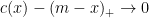
The optimal bound (1) and measure ${\mu^*}$ are easily understood a bit of graphical help. For now, and for the remainder of the post, I fix ${\mu}$ to be a measure on ${{\mathbb R}}$ with ${\int\lvert x\rvert\,d\mu(x) < \infty}$ , let its mean be ${m=\int x\,d\mu(x)}$ , and ${\mu^*}$ be its Hardy-Littlewood transform (2). The measure ${\mu}$ can be represented by a function

$\displaystyle \setlength\arraycolsep{2pt} \begin{array}{rl} &\displaystyle c\colon{\mathbb R}\rightarrow{\mathbb R},\smallskip\\ &\displaystyle c(x)=\int(y-x)_+\,d\mu(y). \end{array}$

This is a non-negative, convex and decreasing function of x. Also, Jensen’s inequality shows that ${c(x)\ge(m-x)_+}$ , and an application of dominated convergence gives the limit

$\displaystyle c(x)-(m-x)_+\rightarrow0$

as ${\lvert x\rvert\rightarrow\infty}$ . If ${X_t}$ has distribution ${\mu}$ then (1) becomes

$\displaystyle {\mathbb P}(X^*_t > x)\le\inf_{y < x}c(y)/(x-y).$

See Figure 1. The right hand side is equal to the absolute gradient of the line passing through ${(x,0)}$ and ${(y,c(y))}$ . The minimum is attained precisely when the curve is a tangent to c, which always occurs for some ${y < x}$ , so long as ${x > m}$ and ${c(x) > 0}$ . If the minimum occurs at ${y=\varphi(x)}$ , then the link between the martingale and its maximum in the optimal case is given by ${X_t=\varphi(X^*_t)}$ .

Alternatively, as c is convex then it has a left (and right) hand derivative everywhere, denoted by ${c^\prime(x-)}$ . A tangent at x is given by the line ${y\mapsto c(x)+(y-x)c^\prime(x-)}$ . This crosses the x-axis at the point

$\displaystyle \Psi(x)\equiv\begin{cases} x-\frac{c(x)}{c^\prime(x-)},&{\rm if\ }c(x) > 0,\\ x,&{\rm if\ }c(x)=0. \end{cases}$

(3)

We note here that the convexity of c together with the limit ${c(x)\rightarrow0}$ as ${x\rightarrow\infty}$ ensures that ${c^\prime(x-) < 0}$ whenever ${c(x) > 0}$ . So, ${\Psi}$ is well defined, and is called the barycenter function of ${\mu}$ . It can also be written as

$\displaystyle \Psi(x)=\mu([x,\infty))^{-1}\int_{[x,\infty)}y\,d\mu(y)$

whenever ${\mu([x,\infty)) > 0}$ . This is a left-continuous inverse to ${\varphi}$ , so the relation between the optimal martingale and its maximum is given by ${X^*_t=\Psi(X_t)}$ — at least, when ${\Psi}$ is continuous. More generally, we will have ${\Psi(X_t)\le X^*_t\le\Psi(X_t+)}$ .

Constructing a Cadlag Solution

I will now show how to construct an example of a martingale with specified terminal distribution for which the maximum attains the optimal bound described by Theorem 1. We may as well fix the terminal time to be at ${t=1}$ , so we do this now. To start with, I give a non-continuous example and leave the construction of a continuous martingale for later. The example given here is interesting in its own right, and is a relatively straightforward construction which is useful in practice for constructing martingales with specified terminal law.

To start, we can state conditions on the martingale for the optimal maximum to be attained. These conditions can be obtained simply by going through the proof of Theorem 1 above and checking when each of the inequalities can be replaced by equality. In the following, ${\varphi}$ is allowed to be ${-\infty}$ because, when the law of ${X_1}$ is unbounded below, then it can be seen that ${\varphi(x)\rightarrow-\infty}$ as ${x\rightarrow m}$ , so we must take ${\varphi(m)=-\infty}$ in order for it to be increasing. This is not a problem because we will always have ${X^*_1 > m}$ (a.s.) whenever ${X_1}$ is not deterministic.

Lemma 5 Let ${\{X_t\}_{t\in[0,1]}}$ be a cadlag martingale satisfying

${X_0=m}$ almost surely.

${X^*_t}$ is continuous.

${X_1=\varphi(X^*_1)}$ (a.s.) for an increasing function ${\varphi\colon[m,\infty)\rightarrow{\mathbb R}\cup\{-\infty\}}$ with ${\varphi(x) > -\infty}$ for all ${x > m}$ .

Then, ${\mu_{X_1^*}=\mu^*_{X_1}}$ .

Proof: Choosing any ${x\in{\mathbb R}}$ , we need to show that ${{\mathbb P}(X^*_1\ge x)}$ achieves the upper bound (1). First, if ${x\le m}$ then we have ${X^*_1\ge X_0\ge x}$ , so the probability is equal to 1 in (1), as required. We just need to consider ${x > m}$ . As ${X_1\le X^*_1}$ , replacing ${\varphi(x)}$ by ${\varphi(x)\wedge x}$ if necessary, we can suppose that ${\varphi(x)\le x}$ .

Let ${\tau}$ be the stopping time

$\displaystyle \tau = \inf\left\{t\in[0,1]\colon X_t\ge x\right\}\cup\{1\}.$

By continuity of ${X^*}$ , we have ${X_\tau\le x}$ . If ${X^*_1 < x}$ then ${\tau=1}$ and ${X_\tau\le\varphi(x)}$ . So,

$\displaystyle {\mathbb P}(X^*_1 \ge x)\ge{\mathbb E}[(X_\tau-\varphi(x))_+]/(x-\varphi(x)).$

Now, if ${\tau < 1}$ then ${X_1=\varphi(X^*_1)\ge\varphi(x)}$ . So, applying the martingale property to ${X-\varphi(x)}$ ,

$\displaystyle (X_\tau-\varphi(x))_+={\mathbb E}[(X_1-\varphi(x))_+\;\vert\mathcal{F}_\tau].$

Taking expectations,

$\displaystyle {\mathbb P}(X^*_1\ge x)\ge\frac{{\mathbb E}[(X_1-\varphi(x))_+]}{x-\varphi(x)}$

as required. ⬜

Now, we move on to a construction. Start with any probability space ${(\Omega,\mathcal{F},{\mathbb P})}$ on which there exists a random variable U with the uniform law on ${(0,1)}$ . Define the filtration

$\displaystyle \mathcal{F}_t=\sigma\left(U1_{\{1-U\le t\}}\right).$

Next, choose any decreasing integrable function ${h\colon(0,1)\rightarrow{\mathbb R}}$ and define the running average, ${\bar h\colon(0,1]\rightarrow{\mathbb R}}$ , as

$\displaystyle \bar h(t)=\frac1t\int_0^th(s)\,ds.$

(4)

Now, we define the cadlag process

$\displaystyle X_t = \begin{cases} \bar h(1-t),&\textrm{if }t <1-U,\\ h(U),&\textrm{if }t\ge1-U. \end{cases}$

(5)

It can be seen that ${X_t={\mathbb E}[h(U)\vert\mathcal{F}_t]}$ , so that X is a martingale. Its terminal distribution and law are

$\displaystyle \setlength\arraycolsep{2pt} \begin{array}{rl} \displaystyle X_1&\displaystyle=h(U),\smallskip\\ \displaystyle X_1^*&\displaystyle=\bar h(U). \end{array}$

The function h can be chosen such that the terminal law is equal to any distribution ${\mu}$ that we like, by setting

$\displaystyle h(t) = \inf\left\{x\in{\mathbb R}\colon\mu((x,\infty))\le t\right\}.$

Finally, the martingale just constructed does have the optimal maximum law.

Lemma 6 The martingale X constructed above, by (5), satisfies ${\mu_{X_1^*}=\mu^*_{X_1}}$ .

Proof: We just need to show that the conditions of Lemma 5 are satisfied. From the definition,

$\displaystyle X_0=\bar h(1)={\mathbb E}[h(U)]=m.$

Also, since h is decreasing, ${\bar h\ge h}$ is decreasing and,

$\displaystyle X^*_t = \bar h((1-t)\vee U)$

is continuous. To complete the proof, we just need to construct the increasing function ${\varphi}$ such that

$\displaystyle h(t)=\varphi(\bar h(t))$

for all ${t\in(0,1)}$ . As ${h,\bar h}$ are both decreasing, it needs to be shown that h is constant on any interval for which ${\bar h}$ is constant. Replacing ${h(t)}$ by its left-limit ${h(t-)}$ if necessary, we can suppose that h is left-continuous. Then, ${\bar h(t)={\mathbb E}[h(tU)]}$ so, if ${\bar h(s)=\bar h(t)}$ for any ${s < t}$ , then ${{\mathbb E}[h(sU)-h(tU)]=0}$ . As h is left-continuous and decreasing, this means that ${h(su)=h(tu)}$ for almost every ${u\in(0,1)}$ and, therefore, h is constant on the interval ${(0,t]}$ . So, ${h(s)=h(t)}$ is constant over ${s\le t}$ . ⬜

In the construction given here, the martingale X follows the deterministic, continuous and increasing curve ${X_t=X^*_t=f(t)\equiv\bar h(1-t)}$ , up until a stopping time ${\tau}$ , after which ${X_t=\varphi(f(\tau))}$ . See Figure 2. We could have constructed the solution directly from this description, although the construction above from the intermediate function h is useful for describing solutions in practice.

Constructing a Continuous Solution

I will now construct a continuous solution, which will be given by a deterministic time change of stopped Brownian motion. This method has very close connections with the Skorokhod embedding problem. Given a Brownian motion B, this asks for a stopping time ${\tau}$ such that ${B^\tau}$ is a uniformly integrable martingale and ${B_\tau}$ has a prescribed distribution. In fact, the construction I give here is essentially given by the Azema-Yor solution to the stopping problem.

Figure 3: An optimal continuous martingale

The idea is to take a Brownian motion B starting from m and define a stopping time ${\tau}$ to be the first time at which ${B_t\le\varphi(B^*_t)}$ . Equivalently, it can be constructed from the barycenter function (3) by stopping at the first time for which ${\Psi(B_t)\le B^*_t}$ . This ensures that ${B_\tau=\varphi(B^*_\tau)}$ . After a deterministic time-change, say ${X_t=B_{\tau\wedge(t/(1-t))}}$ , this gives a continuous local martingale X satisfying ${X_1=\varphi(X^*_1)}$ as for the cadlag solution above. See Figure 3, where ${\tau^*=\tau/(1+\tau)}$ is the stopping time for the time-changed process. It is possible to derive the law for ${X^*_1}$ and ${X_1}$ from the relation ${X_1=\varphi(X^*_1)}$ so, in particular, they must be the same as for the cadlag solution above. Although this can be done directly, the proof is made significantly easier through the use of Azema-Yor processes. The process M in the following lemma is known as an Azema-Yor process and the result holds for all measurable and locally bounded u, although such generality is unnecessary here.

Lemma 7 (Azema-Yor) Let X be a semimartingale such that ${X^*}$ is continuous and ${u\colon{\mathbb R}\rightarrow{\mathbb R}}$ be continuously differentiable. Then, setting ${U(x)=\int u(x)\,dx}$ , the process

$\displaystyle M_t\equiv U(X^*_t)-u(X^*_t)(X^*_t-X_t)$

is a semimartingale satisfying

$\displaystyle M_t=U(X_0)+\int_0^t u(X^*_s)\,dX_s.$ (6)

In particular, if X is a local martingale then so is M.

Proof: As ${X^*}$ is a continuous increasing process and u is continuously differentiable, ${u(X^*)}$ is a continuous FV process and, so, has zero quadratic variation. Using ${dU(X^*)=u(X^*)\,dX^*}$ , we apply integration by parts,

$\displaystyle \setlength\arraycolsep{2pt} \begin{array}{rl} \displaystyle dM&\displaystyle=u(X^*)\,dX^*-u(X^*)\,d(X^*-X)-(X^*-X)\,du(X^*)\smallskip\\ &\displaystyle =u(X^*)\,dX - (X^*-X)\,du(X^*). \end{array}$

(7)

Next, using the fact that ${u(X^*)}$ is constant over any interval on which ${X\not=X^*}$ , and that ${\{t\colon X^*_t-X_t\not=0\}}$ is a countable union of such intervals gives

$\displaystyle \int(X^*-X)\,du(X^*)=0.$

Putting this back in to (7) gives (6) as required. Finally, if X is a cadlag local martingale then, as ${u(X^*)}$ is locally bounded, equation (6) shows that M is also a local martingale. ⬜

Now, we show that the law of the maximum of a martingale can be derived from the relation ${X_1=\varphi(X^*_1)}$ . In the following, in order to handle the case where we do not yet know that X is is a proper martingale, rather than just a local martingale, we also impose the condition that ${X_t\ge\varphi(X^*_t)}$ . It can be seen that this follows from the first condition, so is redundant, whenever X is a proper martingale.

Lemma 8 Let ${\{X\}_{t\in[0,1]}}$ be a cadlag local martingale such that ${X_0=m}$ (a.s.) and ${X^*}$ is continuous. Suppose that ${\varphi\colon[m,\infty)\rightarrow{\mathbb R}\cup\{-\infty\}}$ is increasing with ${x\ge\varphi(x) > -\infty}$ for ${x > m}$ and,

${X_1=\varphi(X^*_1)}$ (a.s.),

${X_t\ge\varphi(X^*_t)}$ (a.s.) for all t.

Then, ${F^*(x)\equiv{\mathbb P}(X^*_1 > x)}$ is the unique right-continuous function satisfying the ODE

$\displaystyle (x-\varphi(x))\,dF^*(x)=-F^*(x)\,dx$ (8)

for ${x\ge m}$ , and ${F^*(x)=1}$ for ${x < m}$ .

Proof: The condition that ${X_0=m}$ immediately gives ${F^*(x)=1}$ for ${x < m}$ . For any twice continuously differentiable ${u\colon{\mathbb R}\rightarrow{\mathbb R}}$ with compact support in ${(m,\infty)}$ , set ${U(x)=\int_m^xu(y)\,dy}$ and let M be the local martingale defined in Lemma 7. As ${\lvert u\rvert}$ is bounded by some ${K > 0}$ and has support in ${[a,b]}$ for some ${b > a > m}$ ,

$\displaystyle \lvert u(X^*)(X^*-X)\rvert\le K(b-\varphi(a))$

is bounded. Hence, M is uniformly bounded, and is a proper martingale. Therefore ${{\mathbb E}[M_1]=0}$ and,

$\displaystyle {\mathbb E}[u(X^*_1)(X^*_1-X_1)]={\mathbb E}[U(X^*_1)].$

On the left hand side, we substitute in ${X_1=\varphi(X^*_1)}$ and use the fact that the law of ${X^*_1}$ is given by ${-\int\cdot\,dF^*(x)}$ . On the right, we replace ${U(X^*)}$ by ${\int u(x)1_{\{X^* > x\}}\,dx}$ to obtain,

$\displaystyle -\int u(x)(x-\varphi(x))\,dF^*(x) = \int u(x)F^*(x)\,dx.$

This proves (8) over ${x > m}$ . Stopping X as soon as it exceeds m gives a bounded martingale and, taking expected values gives

$\displaystyle m{\mathbb P}(X^*_1 > m)+\varphi(m){\mathbb P}(X_1^*=m)=m.$

Rearranging,

$\displaystyle (m-\varphi(m))(1-F^*(m))=0$

and, so, (8) holds for ${x=m}$ .

Finally, suppose that G is another solution to (8) over ${x\ge m}$ with ${G(x)=1}$ for ${x < m}$ . Setting ${H=F^*-G}$ then ${H(x)=0}$ over ${x < m}$ and,

$\displaystyle (x-\varphi(x))dH(x)=-H(x)\,dx$

over ${x\ge m}$ . As ${x-\varphi(x)}$ is nonnegative, this implies that ${\lvert H\rvert}$ is decreasing, so it is identically zero, and the solution ${G=F^*}$ is unique. ⬜

I can now describe a continuous martingale and prove that it has the required terminal and maximum distribution. To start, we define an increasing function ${\varphi\colon[m,\infty)\rightarrow{\mathbb R}\cup\{-\infty\}}$ . The idea, as explained above, is that ${y=\varphi(x) < x}$ is chosen to maximise ${c(y)/(x-y)}$ whenever ${c(x) > 0}$ . In order to obtain a quick proof making use of the cadlag martingale construction above, it will be more convenient to choose ${\varphi}$ as in the proof of Lemma 6 above. We first let ${h\colon(0,1)\rightarrow{\mathbb R}}$ be a decreasing function such that ${h(U)}$ has distribution ${\mu}$ for uniformly distributed random variables U on ${(0,1)}$ , and let ${\bar h}$ be its running average (4). Without loss of generality, we take h to be left-continuous. As explained in the proof of Lemma 6, we can write h as a function of ${\bar h}$ ,

$\displaystyle \varphi(\bar h(t))=h(t).$

This uniquely defines ${\varphi}$ as a right-continuous and increasing function on the image of h. It can be seen that ${y=\varphi(x)}$ does indeed maximise ${c(y)/(x-y)}$ , although I will not use this fact in the proof. We can extend ${\varphi}$ to all of ${[m,\infty)}$ by setting ${\varphi(m)=\inf h}$ and, for ${x\ge\sup\bar h}$ , set ${\varphi(x)=\sup h}$ . Then, ${\varphi(x)\le x}$ is right-continuous and increasing.

Now, let B be a standard Brownian motion defined on some filtered probability space ${(\Omega,\mathcal{F},\{\mathcal{F}_t\}_{t\in{\mathbb R}_+},{\mathbb P})}$ , and starting from ${B_0=m}$ . Define the stopping time

$\displaystyle \tau=\inf\left\{t\ge0\colon B_t\le\varphi(B^*_t)\right\}.$

The recurrence of Brownian motion implies that ${\tau}$ is almost surely finite. Indeed, for any ${t > 0}$ , we have ${B^*_t > m}$ and, so, ${\varphi(B^*_t)}$ is finite. Hence, ${B_s \le \varphi(B^*_t)}$ for some ${s\ge t}$ , with probability 1, and ${\tau\le s}$ . Next, continuity of B ensures that ${B_\tau=\varphi(B^*_\tau)}$ and ${B_{t\wedge\tau}\ge\varphi(B^*_{t\wedge\tau})}$ for all t.

Apply the deterministic time-change

$\displaystyle X_t=B_{\tau\wedge (t/(1-t))}$

over ${t\in[0,1]}$ (in particular, ${X_1=B_\tau}$ ). Then, by the martingale property for the stopped process ${B^\tau}$ , ${X_t}$ will be a martingale with respect to the time-changed filtration

$\displaystyle \mathcal{G}_t=\mathcal{F}_{t/(1-t)}$

over ${t < 1}$ . As ${X_t\rightarrow X_1}$ as ${t\rightarrow1}$ , X is a continuous local martingale.

Finally, I show that X is a martingale with the required terminal and maximum distributions.

Lemma 9 The process X is a proper martingale with ${\mu_{X_1}=\mu}$ and ${\mu_{X_1^*}=\mu^*}$ .

Proof: By Lemma 8, the distribution of ${X^*_1}$ , and hence of ${X_1=\varphi(X^*_1)}$ , is uniquely determined by the property that X is a local martingale with ${X_0=m}$ , ${X_1=\varphi(X^*_1)}$ , and ${X_t\ge\varphi(X^*_t)}$ . So, they are the same as for the solution given by (5), for which ${\mu_{X_1}=\mu}$ and, by Lemma 6, ${\mu_{X_1^*}=\mu^*}$ .

It only remains to prove that X is a proper martingale. Choosing ${t\in(0,1)}$ , We have ${X_s\ge\varphi(X^*_t)}$ over ${s\ge t}$ . As ${X_s-\varphi(X^*_t)}$ is a nonnegative local martingale over ${s\ge t}$ , it is a supermartingale,

$\displaystyle X_t\ge{\mathbb E}[X_1\;\vert\mathcal{G}_t].$

However, we know that ${X_1}$ has distribution ${\mu}$ , so has mean m. Also, as ${X_t}$ is a proper martingale over ${t < 1}$ with ${X_0=m}$ , ${X_t}$ also has mean m. This implies that

$\displaystyle X_t-{\mathbb E}[X_1\;\vert\mathcal{G}_t].$

is nonnegative with zero mean. Hence, X is a proper martingale. ⬜

References

Azéma, J., and Yor, M. (1979) Une solution simple au problème de Skorokhod. Séminaire de Probabilités XIII, Lecture Notes in Math. Vol. 721, 90–115. doi:10.1007/BFb0070852
Azéma, J., and Yor, M. (1979) Le problème de Skorokhod: Compléments à “Une solution simple au problème de Skorokhod”. Séminaire de Probabilités XIII, Lecture Notes in Math. Vol. 721, 625–633. doi:10.1007/BFb0070901
Blackwell, D., and Dubins, L.E. (1963) A converse to the dominated convergence theorem. Illinois J. Math. Vol. 7, no. 3, 508–514. link.
Brown, H., Hobson, D.G., and Rogers, L.C.G. (2001) The maximum maximum of a martingale constrained by an intermediate law. Probab. Theory Related Fields, Vol. 119, 558–578. doi:10.1007/PL00008771
Dubins, L.E., and Gilat, D. (1978). On the distribution of maxima of martingales. Proc. Amer. Math. Soc., Vol. 68, 337–338. doi:10.2307/2043117. Also full-text PDF.
Henry-Labordère, P., Obłój, J., Spoida, P., and Touzi, N. (2016) The maximum maximum of a martingale with given n marginals. Annals of Applied Probability, Vol. 26, No. 1, 1-44. doi:10.1214/14-AAP1084. Also available at arXiv:1203.6877.
Hobson, D.G. (1998) The maximum maximum of a martingale. Séminaire de Probabilités XXXII, Vol. 1686, 250–263. doi:10.1007/BFb0101762. Free ps file available from his website.
Hobson, D.G. (1998) Robust hedging of the lookback option. Finance Stoch., Vol. 2, 329–347. doi:10.1007/s007800050044 Free ps file available from his website.

	Harry on Filtrations and Adapted P…
	Anonymous on Analytic Sets
	Daniel on Analytic Sets
	Sid on Martingale Convergence
	northwiz on Preservation of the Local Mart…
	George Lowther on Martingale Convergence
	Sid on Martingale Convergence
	George Lowther on The Burkholder-Davis-Gundy Ine…
	George Lowther on Preservation of the Local Mart…
	northwiz on Preservation of the Local Mart…

The Maximum Maximum of Martingales with Known Terminal Distribution

Constructing a Cadlag Solution

Constructing a Continuous Solution

References

Published by George Lowther

Leave a Reply Cancel reply

Constructing a Cadlag Solution

Constructing a Continuous Solution

References

Like this:

Related

Published by George Lowther

Leave a Reply Cancel reply