The Optimality of Doob’s Maximal Inequality

One of the most fundamental and useful results in the theory of martingales is Doob’s maximal inequality. Use ${X^*_t\equiv\sup_{s\le t}\lvert X_s\rvert}$ to denote the running (absolute) maximum of a process X. Then, Doob’s ${L^p}$ maximal inequality states that, for any cadlag martingale or nonnegative submartingale X and real ${p > 1}$ ,

$\displaystyle \lVert X^*_t\rVert_p\le c_p \lVert X_t\rVert_p$

(1)

with ${c_p=p/(p-1)}$ . Here, ${\lVert\cdot\rVert_p}$ denotes the standard L^p-norm, ${\lVert U\rVert_p\equiv{\mathbb E}[U^p]^{1/p}}$ .

An obvious question to ask is whether it is possible to do any better. That is, can the constant ${c_p}$ in (1) be replaced by a smaller number. This is especially pertinent in the case of small p, since ${c_p}$ diverges to infinity as p approaches 1. The purpose of this post is to show, by means of an example, that the answer is no. The constant ${c_p}$ in Doob’s inequality is optimal. We will construct an example as follows.

Example 1 For any ${p > 1}$ and constant ${1 \le c < c_p}$ there exists a strictly positive cadlag ${L^p}$ -integrable martingale ${\{X_t\}_{t\in[0,1]}}$ with ${X^*_1=cX_1}$ .

For X as in the example, we have ${\lVert X^*_1\rVert_p=c\lVert X_1\rVert_p}$ . So, supposing that (1) holds with any other constant ${\tilde c_p}$ in place of ${c_p}$ , we must have ${\tilde c_p\ge c}$ . By choosing ${c}$ as close to ${c_p}$ as we like, this means that ${\tilde c_p\ge c_p}$ and ${c_p}$ is indeed optimal in (1).

A natural place to start in trying to construct examples for which (1) is close to equality, is with the methods of the previous post. There, it was shown how to construct martingales with specified terminal distribution and with the maximum possible law for the maximum. In that post, ${X^*}$ was used to denote the running maximum of X rather than the absolute maximum but, as I will just construct nonnegative examples here, this is of no consequence.

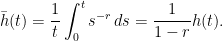
As in the construction of cadlag martingales given in the previous post, start by choosing a (nonnegative) integrable and decreasing function ${h\colon(0,1)\rightarrow{\mathbb R}}$ . Its running average is

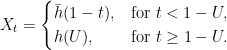
$\displaystyle \bar h(t)=\frac1t\int_0^th(s)\,ds.$

For a random variable U, uniformly distributed on ${(0,1)}$ and defined with respect to a probability space ${(\Omega,\mathcal{F},{\mathbb P})}$ , we construct a cadlag process ${\{X_t\}_{t\in[0,1]}}$ as

$\displaystyle X_t=\begin{cases} \bar h(1-t),&\textrm{for\ }t < 1-U,\\ h(U),&\textrm{for\ }t\ge1-U. \end{cases}$

This is a martingale under its natural filtration, and has the terminal and maximum values,

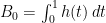
$\displaystyle \setlength\arraycolsep{2pt} \begin{array}{rl} \displaystyle X_1&\displaystyle=h(U),\smallskip\\ \displaystyle X^*_1&\displaystyle=\bar h(U). \end{array}$

Now, it is simple enough to guess at a form for h. Choosing ${h(t)=t^{-r}}$ , this is decreasing for ${r\ge0}$ and integrable for ${r < 1}$ . For X to be ${L^p}$ -integrable, we need ${h(t)^p=t^{-rp}}$ to be integrable, which is true whenever ${r\le1/p}$ . The running average is

$\displaystyle \bar h(t)=\frac1t\int_0^ts^{-r}\,ds= \frac1{1-r}h(t).$

So, ${\bar h=(1-r)^{-1}h}$ and, ${X^*_1 = (1-r)^{-1} X_1}$ . The requirement of the example is satisfied so long as ${(1-r)^{-1}=c}$ or, equivalently, ${r=1-1/c}$ . The condition that ${1\le c < c_p}$ implies that ${0\le r < 1/p}$ , so X is an ${L^p}$ -integrable martingale.

Notes

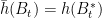
The example constructed above is of a non-continuous martingale. It is not much more difficult to construct a continuous example. As described in the previous post, we can let B be a standard Brownian motion with initial value ${B_0=\int_0^1h(t)\,dt}$ and stopped at the first time for which ${\bar h(B_t)=h(B^*_t)}$ . For the example above, this is the first time at which ${cB_t=B^*_t}$ . This gives a uniformly integrable martingale defined over ${t\in{\mathbb R}_+}$ with ${X^*_\infty=cX_\infty}$ . Applying a deterministic time change gives a martingale ${X_{t/(1-t)}}$ defined over ${t\in[0,1]}$ .

The post on Doob’s inequalities also included the inequality

$\displaystyle {\mathbb P}(X^*_t\ge K)\le\frac1K{\mathbb E}[X^*_t].$

(2)

However, it is easy to see that this is optimal. For any ${K > 0}$ and ${0 < p\le 1}$ , consider a martingale such that ${X_1=K}$ with probability ${p}$ and ${X_1=0}$ with probability ${1-p}$ . Then, (2) is an equality.

	Harry on Filtrations and Adapted P…
	Anonymous on Analytic Sets
	Daniel on Analytic Sets
	Sid on Martingale Convergence
	northwiz on Preservation of the Local Mart…
	George Lowther on Martingale Convergence
	Sid on Martingale Convergence
	George Lowther on The Burkholder-Davis-Gundy Ine…
	George Lowther on Preservation of the Local Mart…
	northwiz on Preservation of the Local Mart…

The Optimality of Doob’s Maximal Inequality

Notes

Published by George Lowther

Leave a Reply Cancel reply

Notes

Like this:

Related

Published by George Lowther

Leave a Reply Cancel reply