Properties of the Dual Projections

In the previous post I introduced the definitions of the dual optional and predictable projections, firstly for processes of integrable variation and, then, generalised to processes which are only required to be locally (or prelocally) of integrable variation. We did not look at the properties of these dual projections beyond the fact that they exist and are uniquely defined, which are significant and important statements in their own right.

To recap, recall that an IV process, A, is right-continuous and such that its variation

$\displaystyle V_t\equiv \lvert A_0\rvert+\int_0^t\,\lvert dA\rvert$

(1)

is integrable at time ${t=\infty}$ , so that ${{\mathbb E}[V_\infty] < \infty}$ . The dual optional projection is defined for processes which are prelocally IV. That is, A has a dual optional projection ${A^{\rm o}}$ if it is right-continuous and its variation process is prelocally integrable, so that there exist a sequence ${\tau_n}$ of stopping times increasing to infinity with ${1_{\{\tau_n > 0\}}V_{\tau_n-}}$ integrable. More generally, A is a raw FV process if it is right-continuous with almost-surely finite variation over finite time intervals, so ${V_t < \infty}$ (a.s.) for all ${t\in{\mathbb R}^+}$ . Then, if a jointly measurable process ${\xi}$ is A-integrable on finite time intervals, we use

$\displaystyle \xi\cdot A_t\equiv\xi_0A_0+\int_0^t\xi\,dA$

to denote the integral of ${\xi}$ with respect to A over the interval ${[0,t]}$ , which takes into account the value of ${\xi}$ at time 0 (unlike the integral ${\int_0^t\xi\,dA}$ which, implicitly, is defined on the interval ${(0,t]}$ ). In what follows, whenever we state that ${\xi\cdot A}$ has any properties, such as being IV or prelocally IV, we are also including the statement that ${\xi}$ is A-integrable so that ${\xi\cdot A}$ is a well-defined process. Also, whenever we state that a process has a dual optional projection, then we are also implicitly stating that it is prelocally IV.

From theorem 3 of the previous post, the dual optional projection ${A^{\rm o}}$ is the unique prelocally IV process satisfying

$\displaystyle {\mathbb E}[\xi\cdot A^{\rm o}_\infty]={\mathbb E}[{}^{\rm o}\xi\cdot A_\infty]$

for all measurable processes ${\xi}$ with optional projection ${{}^{\rm o}\xi}$ such that ${\xi\cdot A^{\rm o}}$ and ${{}^{\rm o}\xi\cdot A}$ are IV. Equivalently, ${A^{\rm o}}$ is the unique optional FV process such that

$\displaystyle {\mathbb E}[\xi\cdot A^{\rm o}_\infty]={\mathbb E}[\xi\cdot A_\infty]$

for all optional ${\xi}$ such that ${\xi\cdot A}$ is IV, in which case ${\xi\cdot A^{\rm o}}$ is also IV so that the expectations in this identity are well-defined.

I now look at the elementary properties of dual optional projections, as well as the corresponding properties of dual predictable projections. The most important property is that, according to the definition just stated, the dual projection exists and is uniquely defined. By comparison, the properties considered in this post are elementary and relatively easy to prove. So, I will simply state a theorem consisting of a list of all the properties under consideration, and will then run through their proofs. Starting with the dual optional projection, the main properties are listed below as Theorem 1.

Note that the first three statements are saying that the dual projection is indeed a linear projection from the prelocally IV processes onto the linear subspace of optional FV processes. As explained in the previous post, by comparison with the discrete-time setting, the dual optional projection can be expressed, in a non-rigorous sense, as taking the optional projection of the infinitesimal increments,

$\displaystyle dA^{\rm o}={}^{\rm o}dA.$

(2)

As ${dA}$ is interpreted via the Lebesgue-Stieltjes integral ${\int\cdot\,dA}$ , it is a random measure rather than a real-valued process. So, the optional projection of ${dA}$ appearing in (2) does not really make sense. However, Theorem 1 does allow us to make sense of (2) in certain restricted cases. For example, if A is differentiable so that ${dA=\xi\,dt}$ for a process ${\xi}$ , then (9) below gives ${dA={}^{\rm o}\xi\,dt}$ . This agrees with (2) so long as ${{}^{\rm o}(\xi\,dt)}$ is interpreted to mean ${{}^{\rm o}\xi\,dt}$ . Also, restricting to the jump component of the increments, ${\Delta A=A-A_-}$ , (2) reduces to (11) below.

We defined the dual projection via expectations of integrals ${\xi\cdot A}$ with the restriction that this is IV. An alternative approach is to first define the dual projections for IV processes, as was done in theorems 1 and 2 of the previous post, and then extend to (pre)locally IV processes by localisation of the projection. That this is consistent with our definitions follows from the fact that (pre)localisation commutes with the dual projection, as stated in (10) below.

Theorem 1

A raw FV process A is optional if and only if ${A^{\rm o}}$ exists and is equal to A.
If the dual optional projection of A exists then,

$\displaystyle (A^{\rm o})^{\rm o}=A^{\rm o}.$ (3)

If the dual optional projections of A and B exist, and ${\lambda}$ , ${\mu}$ are ${\mathcal F_0}$ -measurable random variables then,

$\displaystyle (\lambda A+\mu B)^{\rm o}=\lambda A^{\rm o}+\mu B^{\rm o}.$ (4)

If the dual optional projection ${A^{\rm o}}$ exists then ${{\mathbb E}[\lvert A_0\rvert\,\vert\mathcal F_0]}$ is almost-surely finite and

$\displaystyle A^{\rm o}_0={\mathbb E}[A_0\,\vert\mathcal F_0].$ (5)

If U is a random variable and ${\tau}$ is a stopping time, then ${U1_{[\tau,\infty)}}$ is prelocally IV if and only if ${{\mathbb E}[1_{\{\tau < \infty\}}\lvert U\rvert\,\vert\mathcal F_\tau]}$ is almost surely finite, in which case

$\displaystyle \left(U1_{[\tau,\infty)}\right)^{\rm o}={\mathbb E}[1_{\{\tau < \infty\}}U\,\vert\mathcal F_\tau]1_{[\tau,\infty)}.$ (6)

If the prelocally IV process A is nonnegative and increasing then so is ${A^{\rm o}}$ and,

$\displaystyle {\mathbb E}[\xi\cdot A^{\rm o}_\infty]={\mathbb E}[{}^{\rm o}\xi\cdot A_\infty]$ (7)

for all nonnegative measurable ${\xi}$ with optional projection ${{}^{\rm o}\xi}$ . If A is merely increasing then so is ${A^{\rm o}}$ and (7) holds for nonnegative measurable ${\xi}$ with ${\xi_0=0}$ .

If A has dual optional projection ${A^{\rm o}}$ and ${\xi}$ is an optional process such that ${\xi\cdot A}$ is prelocally IV then, ${\xi}$ is ${A^{\rm o}}$ -integrable and,

$\displaystyle (\xi\cdot A)^{\rm o}=\xi\cdot A^{\rm o}.$ (8)

If A is an optional FV process and ${\xi}$ is a measurable process with optional projection ${{}^{\rm o}\xi}$ such that ${\xi\cdot A}$ is prelocally IV then, ${{}^{\rm o}\xi}$ is A-integrable and,

$\displaystyle (\xi\cdot A)^{\rm o}={}^{\rm o}\xi\cdot A.$ (9)

If A has dual optional projection ${A^{\rm o}}$ and ${\tau}$ is a stopping time then,

$\displaystyle \setlength\arraycolsep{2pt} \begin{array}{rl} &\displaystyle(A^{\tau})^{\rm o}=(A^{\rm o})^{\tau},\smallskip\\ &\displaystyle(A^{\tau-})^{\rm o}=(A^{\rm o})^{\tau-}. \end{array}$ (10)

If the dual optional projection ${A^{\rm o}}$ exists, then its jump process is the optional projection of the jump process of A,

$\displaystyle \Delta A^{\rm o}={}^{\rm o}\!\Delta A.$ (11)

If A has dual optional projection ${A^{\rm o}}$ then

$\displaystyle \setlength\arraycolsep{2pt} \begin{array}{rl} &\displaystyle{\mathbb E}\left[\xi_0\lvert A^{\rm o}_0\rvert + \int_0^\infty\xi\,\lvert dA^{\rm o}\rvert\right]\le{\mathbb E}\left[{}^{\rm o}\xi_0\lvert A_0\rvert + \int_0^\infty{}^{\rm o}\xi\,\lvert dA\rvert\right],\smallskip\\ &\displaystyle{\mathbb E}\left[\xi_0(A^{\rm o}_0)_+ + \int_0^\infty\xi\,(dA^{\rm o})_+\right]\le{\mathbb E}\left[{}^{\rm o}\xi_0(A_0)_+ + \int_0^\infty{}^{\rm o}\xi\,(dA)_+\right],\smallskip\\ &\displaystyle{\mathbb E}\left[\xi_0(A^{\rm o}_0)_- + \int_0^\infty\xi\,(dA^{\rm o})_-\right]\le{\mathbb E}\left[{}^{\rm o}\xi_0(A_0)_- + \int_0^\infty{}^{\rm o}\xi\,(dA)_-\right], \end{array}$ (12)

for all nonnegative measurable ${\xi}$ with optional projection ${{}^{\rm o}\xi}$ .

Let ${\{A^n\}_{n=1,2,\ldots}}$ be a sequence of right-continuous processes with variation
$\displaystyle V^n_t=\lvert A^n_0\rvert + \int_0^t\lvert dA^n\rvert.$

If ${\sum_n V^n}$ is prelocally IV then,

$\displaystyle \left(\sum\nolimits_n A^n\right)^{\rm o}=\sum\nolimits_n\left(A^n\right)^{\rm o}.$ (13)

The proofs of these statements are all relatively direct applications of the definition of the dual optional projection but, as it is a rather long list, I leave the proof until later and, instead, move directly on to the properties of dual predictable projections. Recall that a process A is locally IV if there exists a sequence ${\tau_n}$ of stopping times increasing to infinity such that ${1_{\{\tau_n > 0\}}A^{\tau_n}}$ are IV. For such a process, its dual predictable projection ${A^{\rm p}}$ is the unique locally IV process satisfying

$\displaystyle {\mathbb E}[\xi\cdot A^{\rm p}_\infty]={\mathbb E}[{}^{\rm p}\cdot A_\infty]$

for all measurable ${\xi}$ with predictable projection ${{}^{\rm p}\xi}$ such that ${\xi\cdot A^{\rm p}}$ and ${{}^{\rm p}\xi\cdot A}$ are IV. Equivalently, ${A^{\rm p}}$ is the unique predictable FV process such that

$\displaystyle {\mathbb E}[\xi\cdot A^{\rm p}_\infty]={\mathbb E}[\xi\cdot A_\infty]$

for all predictable ${\xi}$ such that ${\xi\cdot A}$ is IV, in which case ${\xi\cdot A^{\rm p}}$ is also IV.

The list of properties stated in Theorem 1 above carry across to the dual predictable projection. The only significant difference here is the addition of an extra property in statement 13 below, which interprets the dual predictable projection of an adapted locally IV process as its compensator.

Below, whenever we state that the dual predictable projection of a process A exists then we are implicitly also saying that A is locally IV.

Theorem 2

A raw FV process A is predictable if and only if ${A^{\rm p}}$ exists and is equal to A.
If the dual predictable projection of A exists then,

$\displaystyle (A^{\rm p})^{\rm p}=A^{\rm p}.$ (14)

If the dual predictable projections of A and B exist, and ${\lambda}$ , ${\mu}$ are ${\mathcal F_0}$ -measurable random variables then,

$\displaystyle (\lambda A+\mu B)^{\rm p}=\lambda A^{\rm p}+\mu B^{\rm p}.$ (15)

If the dual predictable projection ${A^{\rm p}}$ exists then ${{\mathbb E}[\lvert A_0\rvert\,\vert\mathcal F_0]}$ is almost-surely finite and

$\displaystyle A^{\rm p}_0={\mathbb E}[A_0\,\vert\mathcal F_0].$ (16)

If U is a random variable and ${\tau}$ is a predictable stopping time, then ${U1_{[\tau,\infty)}}$ is locally IV if and only if ${{\mathbb E}[1_{\{\tau < \infty\}}\lvert U\rvert\,\vert\mathcal F_{\tau-}]}$ is almost surely finite, in which case

$\displaystyle \left(U1_{[\tau,\infty)}\right)^{\rm p}={\mathbb E}[1_{\{\tau < \infty\}}U\,\vert\mathcal F_{\tau-}]1_{[\tau,\infty)}.$ (17)

If the locally IV process A is nonnegative and increasing then so is ${A^{\rm p}}$ and,

$\displaystyle {\mathbb E}[\xi\cdot A^{\rm p}_\infty]={\mathbb E}[{}^{\rm p}\xi\cdot A_\infty]$ (18)

for all nonnegative measurable ${\xi}$ with predictable projection ${{}^{\rm p}\xi}$ . If A is merely increasing then so is ${A^{\rm p}}$ and (18) holds for nonnegative measurable ${\xi}$ with ${\xi_0=0}$ .

If A has dual predictable projection ${A^{\rm p}}$ and ${\xi}$ is a predictable process such that ${\xi\cdot A}$ is locally IV then, ${\xi}$ is ${A^{\rm p}}$ -integrable and,

$\displaystyle (\xi\cdot A)^{\rm p}=\xi\cdot A^{\rm p}.$ (19)

If A is a predictable FV process and ${\xi}$ is a measurable process with predictable projection ${{}^{\rm p}\xi}$ such that ${\xi\cdot A}$ is locally IV then, ${{}^{\rm p}\xi}$ is A-integrable and,

$\displaystyle (\xi\cdot A)^{\rm p}={}^{\rm p}\xi\cdot A.$ (20)

If A has dual predictable projection ${A^{\rm p}}$ and ${\tau}$ is a stopping time then,

$\displaystyle (A^{\tau})^{\rm p}=(A^{\rm p})^{\tau}.$ (21)

If ${\tau}$ is a predictable stopping time then,

$\displaystyle (A^{\tau-})^{\rm p}=(A^{\rm p})^{\tau-}.$ (22)

If the dual predictable projection ${A^{\rm p}}$ exists, then its jump process is the predictable projection of the jump process of A,

$\displaystyle \Delta A^{\rm p}={}^{\rm p}\!\Delta A.$ (23)

If A has dual predictable projection ${A^{\rm p}}$ then

$\displaystyle \setlength\arraycolsep{2pt} \begin{array}{rl} &\displaystyle{\mathbb E}\left[\xi_0\lvert A^{\rm p}_0\rvert + \int_0^\infty\xi\,\lvert dA^{\rm p}\rvert\right]\le{\mathbb E}\left[{}^{\rm p}\xi_0\lvert A_0\rvert + \int_0^\infty{}^{\rm p}\xi\,\lvert dA\rvert\right],\smallskip\\ &\displaystyle{\mathbb E}\left[\xi_0(A^{\rm p}_0)_+ + \int_0^\infty\xi\,(dA^{\rm p})_+\right]\le{\mathbb E}\left[{}^{\rm p}\xi_0(A_0)_+ + \int_0^\infty{}^{\rm p}\xi\,(dA)_+\right],\smallskip\\ &\displaystyle{\mathbb E}\left[\xi_0(A^{\rm p}_0)_- + \int_0^\infty\xi\,(dA^{\rm p})_-\right]\le{\mathbb E}\left[{}^{\rm p}\xi_0(A_0)_- + \int_0^\infty{}^{\rm p}\xi\,(dA)_-\right], \end{array}$ (24)

for all nonnegative measurable ${\xi}$ with predictable projection ${{}^{\rm p}\xi}$ .

Let ${\{A^n\}_{n=1,2,\ldots}}$ be a sequence of right-continuous processes with variation
$\displaystyle V^n_t=\lvert A^n_0\rvert + \int_0^t\lvert dA^n\rvert.$

If ${\sum_n V^n}$ is locally IV then,

$\displaystyle \left(\sum\nolimits_n A^n\right)^{\rm p}=\sum\nolimits_n\left(A^n\right)^{\rm p}.$ (25)

If A is an adapted locally IV process then ${A^{\rm p}}$ is the unique predictable FV process such that ${A-A^{\rm p}}$ is a local martingale starting from 0.

As with Theorem 1, we leave the proof of the above until further down in this post. For now, we show the following property combining the dual optional and projections.

Theorem 3 Let A be locally an IV process. Then, ${A^{\rm o}}$ is locally IV and

$\displaystyle (A^{\rm o})^{\rm p}=(A^{\rm p})^{\rm o}=A^{\rm p}.$

Proof: As A is locally IV, there exists a sequence ${\tau_n}$ of stopping times increasing to infinity such that ${1_{\{\tau_n > 0\}}A^{\tau_n}}$ are IV. So, A is prelocally IV and, from (10),

$\displaystyle 1_{\{\tau_n > 0\}}(A^{\rm o})^{\tau_n}=\left(1_{\{\tau_n > 0\}}A^{\tau_n}\right)^{\rm o}$

is IV. So, ${A^{\rm o}}$ is locally IV. If ${\xi}$ is a predictable process such that ${\xi\cdot A}$ is IV, then ${\xi\cdot A^{\rm o}}$ and, hence, ${\xi\cdot(A^{\rm o})^{\rm p}}$ , are IV and,

$\displaystyle {\mathbb E}[\xi\cdot(A^{\rm o})^{\rm p}_\infty] ={\mathbb E}[\xi\cdot A^{\rm o}_\infty] ={\mathbb E}[\xi\cdot A_\infty].$

From the definition, this means that ${(A^{\rm o})^{\rm p}}$ is the dual predictable projection of A. Finally, as ${A^{\rm p}}$ is predictable and, hence, optional, it is equal to its optional projection ${(A^{\rm p})^{\rm o}=A^{\rm p}}$ . ⬜

Finally, the difference between the dual optional and predictable projections is always a local martingale.

Lemma 4 Let A be a locally IV process. Then, ${A^{\rm o}-A^{\rm p}}$ is a local martingale.

Proof: By theorem 3,

$\displaystyle A^{\rm o}-A^{\rm p}=A^{\rm o}-(A^{\rm o})^{\rm p}$

which, by statement 13 of theorem 2, is a local martingale. ⬜

Proof of Theorem 1

I will now go through and prove each of the statements of theorem 1 in turn. It should be noted that the statements all follow quite directly from theorems 1 and 2 of the previous post, so along as all the processes to which optional projection is applied are actually IV and all integrands are bounded. Extending to prelocally IV processes and unbounded integrands can be done in several ways. One method is to choose a localising sequence of stopping times ${\tau_n}$ and apply the results to the prestopped processes ${1_{\{\tau_n > 0\}}A^{\tau_n-}}$ , taking the limit ${n\rightarrow\infty}$ to extend the results to the prelocally IV process A. Dominated convergence can be used to remove the boundedness requirements for the integrands. An alternative approach, which is closer to the definitions we are using for the dual projections, is to choose an optional process ${\beta > 0}$ such that ${\beta\cdot A}$ is IV, in the same way as in the proof of theorem 3 of the previous post. The result for ${\beta\cdot A}$ can be extended to apply to A by simply cancelling out the ${\beta}$ term at the end. We use this approach for statements 6, 7, 8 and 12 below.

Proof of 1: First, by definition, the dual optional projection is optional and so, if ${A=A^{\rm o}}$ , then A is optional. Conversely, suppose that A is an optional FV process. Then it is adapted and so its variation process (1) is also adapted and, hence, is prelocally integrable. This shows that A is prelocally IV so has an optional projection which, from the definition, is equal to A.

Proof of 2: By definition, ${A^{\rm o}}$ is optional and prelocally IV and, hence, is equal to its own dual optional projection.

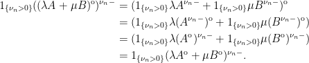
Proof of 3: We start with the case where A and B are IV, and ${\lambda}$ and ${\mu}$ are uniformly bounded. Then, for bounded measurable ${\xi}$ , applying theorem 1 of the previous post,

$\displaystyle \setlength\arraycolsep{2pt} \begin{array}{rl} \displaystyle{\mathbb E}[\xi\cdot(\lambda A^{\rm o}+\mu B^{\rm o})_\infty] &\displaystyle={\mathbb E}[(\lambda\xi)\cdot A^{\rm o}_\infty]+{\mathbb E}[(\mu\xi)\cdot B^{\rm o}_\infty]\smallskip\\ &\displaystyle={\mathbb E}[(\lambda\,{}^{\rm o}\xi)\cdot A_\infty]+{\mathbb E}[(\mu\,{}^{\rm o}\xi)\cdot B_\infty]\smallskip\\ &\displaystyle={\mathbb E}[{}^{\rm o}\xi\cdot(\lambda A+\mu B)_\infty]. \end{array}$

Again, by theorem 1 of the previous post, this implies (4).

We generalise to the case where it is only assumed that A and B are prelocally IV, and ${\lambda}$ and ${\mu}$ are ${\mathcal F_0}$ -measurable. By definition, there exists stopping times ${\sigma_n,\tau_n}$ increasing to infinity as ${n\rightarrow\infty}$ , and such that ${1_{\{\sigma_n > 0\}}A^{\sigma_n-}}$ and ${1_{\{\tau_n > 0\}}A^{\tau_n-}}$ are IV. Also define stopping times ${\upsilon_n=0}$ on ${\{\lvert\lambda\rvert+\lvert\mu\rvert > n\}}$ and ${\upsilon_n=\infty}$ otherwise. Setting ${\nu_n=\sigma_n\wedge\tau_n\wedge\upsilon_n}$ then ${1_{\{\nu_n > 0\}}\lambda}$ and ${1_{\{\nu_n > 0\}}\mu}$ are bounded. We will apply statement 9, which will be proven below, in order to commute the dual optional projection with pre-stopping at time ${\nu_n}$ .

$\displaystyle \setlength\arraycolsep{2pt} \begin{array}{rl} \displaystyle 1_{\{\nu_n > 0\}}((\lambda A+\mu B)^{\rm o})^{\nu_n-} &\displaystyle=(1_{\{\nu_n > 0\}}\lambda A^{\nu_n-}+1_{\{\nu_n > 0\}}\mu B^{\nu_n-})^{\rm o}\smallskip\\ &\displaystyle=(1_{\{\nu_n > 0\}}\lambda (A^{\nu_n-})^{\rm o}+1_{\{\nu_n > 0\}}\mu(B^{\nu_n-})^{\rm o})\smallskip\\ &\displaystyle=(1_{\{\nu_n > 0\}}\lambda (A^{\rm o})^{\nu_n-}+1_{\{\nu_n > 0\}}\mu(B^{\rm o})^{\nu_n-})\smallskip\\ &\displaystyle=1_{\{\nu_n > 0\}}(\lambda A^{\rm o}+\mu B^{\rm o})^{\nu_n-}. \end{array}$

The second equality is an application of (4) for the case proven above. This shows that (4) holds on the interval ${[0,\nu_n)}$ and letting n go to infinity gives the result.

Proof of 4: As A is prelocally IV, ${A_0}$ is integrable with respect to ${\mathcal F_0}$ . Also, as it is optional, ${A^{\rm o}_0}$ is ${\mathcal F_0}$ -measurable. Then, if U is an ${\mathcal F_0}$ -measurable random variable such that ${UA_0}$ is integrable then,

$\displaystyle \setlength\arraycolsep{2pt} \begin{array}{rl} \displaystyle{\mathbb E}[UA^{\rm o}_0] &\displaystyle={\mathbb E}[(U1_{[0]})\cdot A^{\rm o}_\infty]\smallskip\\ &\displaystyle={\mathbb E}[(U1_{[0]})\cdot A_\infty]\smallskip\\ &\displaystyle={\mathbb E}[UA_0]. \end{array}$

By definition of conditional expectations, this is equivalent to (5).

Proof of 5: Writing ${A=U1_{[\tau,\infty)}}$ , if A is prelocally IV then ${A_\tau=1_{\{\tau < \infty\}}U}$ is integrable w.r.t. ${\mathcal F_\tau}$ . So,

$\displaystyle {\mathbb E}[1_{\{\tau < \infty\}}\lvert U\rvert\,\vert\mathcal F_\tau]={\mathbb E}[\lvert A_\tau\rvert\,\vert\mathcal F_\tau] < \infty$

almost surely. Conversely, if ${V\equiv{\mathbb E}[1_{\{\tau < \infty\}}\lvert U\rvert\,\vert\mathcal F_\tau]}$ is almost surely finite, we can define a sequence of stopping times ${\tau_n}$ increasing to infinity by, ${\tau_n=\tau}$ whenever ${V > n}$ and ${\tau_n=\infty}$ when ${V \le n}$ . Then, ${1_{\{\tau_n > 0\}}A^{\tau_n-}}$ has variation bounded by n and, hence, A is prelocally IV.

Writing ${B={\mathbb E}[1_{\{\tau < \infty\}}U\,\vert\mathcal F_\tau]1_{[\tau,\infty)}}$ then, for optional ${\xi}$ ,

$\displaystyle \setlength\arraycolsep{2pt} \begin{array}{rl} \displaystyle{\mathbb E}[\xi\cdot B_\infty] &\displaystyle={\mathbb E}[\xi_\tau{\mathbb E}[1_{\{\tau < \infty\}}U\,\vert\mathcal F_\tau]]\smallskip\\ &\displaystyle={\mathbb E}[{}^{\rm o}\xi_\tau U]={\mathbb E}[{}^{\rm o}\xi\cdot A_\infty] \end{array}$

whenever ${\xi\cdot B}$ and ${{}^{\rm o}\xi\cdot A}$ are IV, showing that ${B=A^{\rm o}}$ .

Proof of 6: Let A be a nonnegative increasing prelocally IV process. By definition, there exists stopping times ${\tau_n}$ increasing to infinity such that ${1_{\{\tau_n > 0\}}A^{\tau_n-}}$ are IV and, by theorem 1 of the previous post, have nonnegative and increasing dual optional projections. We apply statement 9, which will be proven below, in order to commute the dual optional projection with pre-stopping at time ${\tau_n}$ to see that

$\displaystyle 1_{\{\tau_n > 0\}}(A^{\rm o})^{\tau_n-}=(1_{\{\tau_n > 0\}}A)^{\rm o}$

is nonnegative and increasing. Letting n go to infinity shows that ${A^{\rm o}}$ is nonnegative and increasing. We show that (7) holds for nonnegative measurable ${\xi}$ . Although it need not be the case that ${\xi}$ is ${A^{\rm o}}$ integrable or that ${{}^{\rm o}\xi}$ is A-integrable, as the integrals are nonnegative, the expectations in (7) are well-defined although, possibly, infinite. First (7) holds whenever ${\xi\cdot A^{\rm o}}$ and ${{}^{\rm o}\xi\cdot A}$ are integrable, from the definition of the dual optional projection. Furthermore, as A is prelocally IV, there exists an optional ${\beta > 0}$ such that ${\beta\cdot A}$ and, hence, ${\beta\cdot A^{\rm o}}$ are IV. We can approximate ${\xi}$ by a sequence of optional processes ${\xi^n=\xi\wedge(n\beta)}$ . Then, (7) holds with ${\xi^n}$ in place of ${\xi}$ and, ${\xi^n\uparrow\xi}$ . By dominated convergence of optional projections, ${{}^{\rm o}\xi^n\uparrow{}^{\rm o}\xi}$ as n goes to infinity. So, by monotone convergence of the expectations, (7) holds for all nonnegative measurable ${\xi}$ .

Next, suppose that A is increasing but not necessarily nonnegative. Then ${B\equiv A+\lvert A_0\rvert}$ is nonnegative and, applying statement 5 above,

$\displaystyle A^{\rm o}=B^{\rm o}-{\mathbb E}[\lvert A_0\rvert\,\vert\mathcal F_0]$

is increasing. If ${\xi}$ is a nonnegative measurable process with ${\xi_0=0}$ then ${\xi\cdot B^{\rm o}=\xi\cdot A^{\rm o}}$ and, as ${{}^{\rm o}\xi_0=0}$ , we also have ${{}^{\rm o}\xi\cdot B={}^{\rm o}\xi\cdot A}$ . Hence, (7) follows by applying the equality to B.

Proof of 7: As ${\xi\cdot A}$ is prelocally IV, there exists an optional process ${\beta > 0}$ such that ${\beta\cdot(\xi\cdot A)=(\beta\xi)\cdot A}$ is IV. From the definition of the dual optional projection, ${(\beta\xi)\cdot A^{\rm o}}$ is also IV, so, integrating over ${\beta^{-1}}$ shows that ${\xi}$ is A-integrable and,

holds for all bounded measurable ${\zeta}$ . Therefore,

$\displaystyle \beta\cdot(\xi\cdot A)^{\rm o}=(\beta\xi)\cdot A^{\rm o}.$

Integrating ${\beta^{-1}}$ with respect to both sides gives (8).

Proof of 8: As A is optional FV, statement 1 says that it is prelocally IV with dual optional projection ${A^{\rm o}=A}$ . As ${\xi\cdot A}$ is prelocally IV, there exists an optional ${\beta > 0}$ so that ${\beta\cdot(\xi\cdot A)=(\beta\xi)\cdot A}$ is IV. From the definition of the dual optional projection, ${\beta\cdot(\xi\cdot A)^{\rm o}}$ is also IV. Similarly, there is an optional ${\gamma > 0}$ such that ${\gamma\cdot A}$ is IV and, by choosing ${\beta\lvert{}^{\rm o}\xi\rvert\le\gamma}$ we can ensure that ${(\beta\,{}^{\rm o}\xi)\cdot A}$ is IV. Then, applying the definition of the dual optional projection and using ${A^{\rm o}=A}$ gives

$\displaystyle \setlength\arraycolsep{2pt} \begin{array}{rl} \displaystyle{\mathbb E}[(\zeta\beta)\cdot(\xi\cdot A)^{\rm o}_\infty] &\displaystyle={\mathbb E}[({}^{\rm o}\zeta\beta)\cdot(\xi\cdot A)_\infty]\smallskip\\ &\displaystyle={\mathbb E}[({}^{\rm o}\zeta\beta\xi)\cdot A_\infty]\smallskip\\ &\displaystyle={\mathbb E}[{}^{\rm o}({}^{\rm o}\zeta\beta\xi)\cdot A_\infty]\smallskip\\ &\displaystyle={\mathbb E}[{}^{\rm o}(\zeta\beta\,{}^{\rm o}\xi)\cdot A_\infty]\smallskip\\ &\displaystyle={\mathbb E}[(\zeta\beta\,{}^{\rm o}\xi)\cdot A_\infty] \end{array}$

for all bounded measurable ${\zeta}$ . So,

$\displaystyle \beta\cdot(\xi\cdot A)^{\rm o}=(\beta\,{}^{\rm o}\xi)\cdot A.$

Integrating ${\beta^{-1}}$ with respect to both sides gives (9).

Proof of 9: If ${\tau}$ is a stopping time then ${1_{[0,\tau]}}$ is optional (in fact, it is predictable). Applying statement 7 above,

$\displaystyle (A^\tau)^{\rm o}=(1_{[0,\tau]}\cdot A)^{\rm o}=1_{[0,\tau]}\cdot A^{\rm o}=(A^{\rm o})^\tau.$

Similarly, ${\xi\equiv1_{[0,\tau)}+1_{\{\tau=0\}}1_{[0]}}$ is optional and ${A^{\tau-}=\xi\cdot A}$ . Again applying statement 7,

$\displaystyle (A^{\tau-})^{\rm o}=(\xi\cdot A)^{\rm o}=\xi\cdot A^{\rm o}=(A^{\rm o})^{\tau-}.$

as required.

Proof of 10: As A is prelocally IV, ${{\mathbb E}[\lvert\Delta A_\tau\rvert\,\vert\mathcal F_\tau]}$ is almost surely finite for each stopping time ${\tau}$ , so its optional projection exists. Next, as ${A^{\rm o}_-}$ is left-continuous and adapted, it is optional (in fact, it is predictable). So, ${\Delta A^{\rm o}=A^{\rm o}-A^{\rm o}_-}$ is optional. In particular, this means that ${\Delta A^{\rm o}_\tau}$ is ${\mathcal F_\tau}$ -measurable. We procede in a similar fashion as in the proof of statement 4. For any ${\mathcal F_\tau}$ -measurable random variable such that ${U\Delta A_\tau}$ is integrable, then ${\xi\equiv 1_{\{\tau > 0\}}U1_{[\tau]}}$ is optional and,

$\displaystyle \setlength\arraycolsep{2pt} \begin{array}{rl} \displaystyle{\mathbb E}[U\Delta A^{\rm o}_\tau] &\displaystyle={\mathbb E}[(1_{\{\tau > 0\}}U1_{[\tau]})\cdot A^{o}_\infty]\smallskip\\ &\displaystyle={\mathbb E}[(1_{\{\tau > 0\}}U1_{[\tau]})\cdot A_\infty]\smallskip\\ &\displaystyle={\mathbb E}[U\Delta A_\tau] \end{array}$

So, by definition of the conditional expectation, ${{\mathbb E}[\Delta A_\tau\,\vert\mathcal F_\tau]}$ is equal to ${\Delta A^{\rm o}_\tau}$ , showing that ${\Delta A^{\rm o}}$ is the optional projection of ${\Delta A}$ .

Proof of 11: Denoting the increasing part of A by

$\displaystyle B_t\equiv(A_0)_++\int_0^t\,(dA)_+$

then ${B}$ and ${B-A}$ are nonnegative and increasing. By statement 6 above, this means that ${B^{\rm o}}$ and ${B^{\rm o}-A^{\rm o}}$ are nonnegative and increasing. So, ${\xi\cdot B^{\rm o}}$ and ${\xi\cdot B^{\rm o}-\xi\cdot A^{\rm o}}$ is increasing, for nonnegative bounded ${\xi}$ . Denoting the increasing part of ${\xi\cdot A^{\rm o}}$ by

$\displaystyle C_t\equiv \xi_0(A^{\rm o}_0)_++\int_0^t\xi\,(dA^{\rm o})_+$

this means that ${\xi\cdot B^{\rm o}-C}$ is increasing. Taking expectations and applying (7),

$\displaystyle {\mathbb E}[C_\infty]\le{\mathbb E}[\xi\cdot B^{\rm o}_\infty]={\mathbb E}[{}^{\rm o}\xi\cdot B_\infty].$

This proves the second of equalities (12) for bounded ${\xi}$ and, by monotone convergence, shows that it holds for all nonnegative ${\xi}$ . The third equality of (12) follows from the second one applied to ${-A}$ , and the first follows from adding together the second and third ones.

Proof of 12: As ${V^n\pm A^n}$ are nonnegative increasing processes, we have ${\lvert A^n\rvert\le V^n}$ . By the hypothesis of the theorem, ${V\equiv\sum_nV^n}$ is prelocally integrable and, hence,

$\displaystyle \sum\nolimits_n\lvert A^n\rvert\le V,$

so the sum ${A\equiv\sum_nA^n}$ is absolutely convergent and ${V\pm A}$ is increasing. This shows that the variation of A is bounded by V, so A is prelocally IV. Next, by statement 6 above, ${(V^n)^{\rm o}\pm(A^n)^{\rm o}}$ and ${V^{\rm o}-\sum_{n\le m}(V^n)^{\rm o}}$ are nonnegative increasing processes. So,

$\displaystyle \sum\nolimits_n\lvert (A^n)^{\rm o}\rvert\le\sum\nolimits_n (V^n)^{\rm o}\le V^{\rm o}.$

Therefore, ${B\equiv\sum_n(A^n)^{\rm o}}$ is also absolutely convergent. This shows that, at least, both sides of (13) are well-defined. We just need to demonstrate that they are equal. To do this, we make use of the identities

$\displaystyle \setlength\arraycolsep{2pt} \begin{array}{rl} &\displaystyle\xi\cdot A = \sum\nolimits_n\xi\cdot A^n,\smallskip\\ &\displaystyle\xi\cdot B = \sum\nolimits_n\xi\cdot (A^n)^{\rm o}, \end{array}$

For ${\xi}$ of the form ${U1_{[0,T]}}$ , for a random variable U and time ${T\ge0}$ , these are trivial, and extends to arbitrary bounded measurable ${\xi}$ by the functional monotone class theorem. Then, if ${\xi}$ is any bounded process such that ${\xi\cdot V^{\rm o}}$ and ${{}^{\rm o}\xi\cdot V}$ are IV, we have

$\displaystyle \setlength\arraycolsep{2pt} \begin{array}{rl} \displaystyle{\mathbb E}[\xi\cdot A^{\rm o}_\infty] &\displaystyle={\mathbb E}[{}^{\rm o}\xi\cdot A_\infty] ={\mathbb E}\left[\sum\nolimits_n{}^{\rm o}\xi\cdot A^n_\infty\right]\smallskip\\ &\displaystyle=\sum\nolimits_n{\mathbb E}\left[{}^{\rm o}\xi\cdot A^n_\infty\right] =\sum\nolimits_n{\mathbb E}\left[\xi\cdot(A^n)^{\rm o}_\infty\right]\smallskip\\ &\displaystyle={\mathbb E}\left[\sum\nolimits_n\xi\cdot(A^n)^{\rm o}_\infty\right] ={\mathbb E}[\xi\cdot B_\infty]. \end{array}$

In particular, as V is prelocally integrable, there will be a bounded optional ${\beta > 0}$ such that ${\beta\cdot V}$ and, hence, ${\beta\cdot V^{\rm o}}$ are prelocally IV. Then, for any bounded measurable ${\xi}$ , we can apply the identity above with ${\xi\beta}$ in place of ${\xi}$ ,

$\displaystyle {\mathbb E}[(\xi\beta)\cdot A^{\rm o}_\infty]={\mathbb E}[(\xi\beta)\cdot B_\infty].$

As this holds for all bounded measurable ${\xi}$ , we have ${\beta\cdot A^{\rm o}=\beta\cdot B}$ and, integrating over ${\beta^{-1}}$ , gives ${A^{\rm o}=B}$ as required.

Proof of Theorem 2

The first 12 statements of theorem 1 correspond directly to the 12 statements of theorem 1 and, for the main part, the proofs given above carry across directly. We simply replace `optional’ with `predictable’, `prelocally IV’ with `locally IV’, the prestopped process ${1_{\{\tau_n > 0\}}A^{\tau_n-}}$ by the stopped processes ${1_{\{\tau_n > 0\}}A^{\tau_n}}$ , and `stopping time’ by `predictable stopping time’ (and ${\mathcal F_\tau}$ by ${\mathcal F_{\tau-}}$ ) where necessary. Here, I will merely mention the points where the argument does not directly carry across and say how it can be modified.

First, in the proof of statement 1, we used the fact that if A is adapted then so is its variation V which, consequently, is prelocally IV. In the case where A is predictable then, by approximating the variation V along partitions of ${{\mathbb R}^+}$ (see (17) from the previous post), it can be seen that V is also predictable. This is enough to show that V is locally bounded. This fact follows from the fact that, for the stopping times ${\tau_n=\inf\{t\ge0\colon V_t\ge n\}}$ , the stochastic intervals ${[\tau_n,\infty)}$ are equal to ${\{V\ge n\}\in\mathcal P}$ and, hence, ${\tau_n}$ are predictable stopping times. If ${\tau_{n1},\tau_{n2},\ldots}$ announce ${\tau_n}$ , then the stopping times ${\sigma_n=\tau_{1n}\vee\cdots\vee\tau_{nn}}$ are increasing to infinity, and ${1_{\{\sigma_n > 0\}}V^{\sigma_n} \le n}$ . In particular, V is locally integrable as required.

In the proof of statement 5, we showed that, for a stopping time ${\tau}$ and random variable ${V={\mathbb E}[\lvert U\rvert\,\vert\mathcal F_{\tau}]}$ , then the process ${U1_{[\tau,\infty)}}$ is prelocally IV so long as V is almost surely finite. This follows from the fact that ${B\equiv V1_{[\tau,\infty)}}$ is prelocally integrable. In the case where ${\tau}$ is a predictable stopping time and the sigma-algebra ${\mathcal F_\tau}$ is replaced by ${\mathcal F_{\tau-}}$ , then the process B will be an increasing predictable process, so will be locally IV by the argument in the previous paragraph.

In statement 9 of theorem 2, identity (22) only applies when ${\tau}$ is a predictable stopping time, whereas the equivalent statement (10) of theorem 1 applied for all stopping times. This is because they are applications of (8,19) with ${\xi\equiv1_{[0,\tau)}+1_{\{\tau=0\}}1_{[0]}}$ , which is optional for any stopping time ${\tau}$ , but requires ${\tau}$ to be a predictable stopping time for ${\xi}$ to be predictable so that (19) applies.

Finally, statement 13 of theorem 2 does not correspond to any of the statements of theorem 1, so I give a proof here.

Proof of 13: Starting with the case where A is IV, then ${M\equiv A-A^{\rm p}}$ is an adapted process satisfying

$\displaystyle {\mathbb E}\left[\int_0^t\xi\cdot M_\infty\right]={\mathbb E}[\xi\cdot A_\infty]-{\mathbb E}[\xi\cdot A^{\rm p}_\infty]=0$

for bounded predictable ${\xi}$ . In particular, it holds for bounded elementary ${\xi}$ , showing that M is a martingale. Next suppose that A is locally IV. Then, there are stopping times ${\tau_n}$ increasing to infinity such that ${1_{\{\tau_n > 0\}}A^{\tau_n}}$ is IV. Then,

$\displaystyle M^{\tau_n} = 1_{\{\tau_n > 0\}}(A^{\tau_n}-(A^{\tau_n})^{\rm p})$

is a martingale, so M is a local martingale. To show uniqueness, suppose that B is a predictable FV process such that ${A-B}$ is a local martingale starting from zero. Then, ${C\equiv A^{\rm p}-B}$ is a predictable local martingale starting from zero. By the first statement of Theorem 2, C is a locally IV process starting from zero and with dual predictable projection equal to itself. Letting ${\tau_n}$ be a sequence of stopping times increasing to infinity such that ${C^{\tau_n}}$ are IV. Then, as they are class (D) local martingales, ${C^{\tau_n}}$ are proper martingales and hence,

$\displaystyle {\mathbb E}[\xi\cdot C^{\tau_n}_\infty]=0$

for bounded elementary ${\xi}$ . By the functional monotone class theorem, this extends to all bounded predictable ${\xi}$ . Then, as C is its own dual predictable projection,

$\displaystyle {\mathbb E}[\xi\cdot C^{\tau_n}_\infty]={\mathbb E}[{}^{\rm p}\xi\cdot C^{\tau_n}_\infty]=0$

for all bounded measurable ${\xi}$ . So, ${C^{\tau_n}=0}$ and, letting n go to infinity, ${B=A^{\rm p}}$ .

	Harry on Filtrations and Adapted P…
	Anonymous on Analytic Sets
	Daniel on Analytic Sets
	Sid on Martingale Convergence
	northwiz on Preservation of the Local Mart…
	George Lowther on Martingale Convergence
	Sid on Martingale Convergence
	George Lowther on The Burkholder-Davis-Gundy Ine…
	George Lowther on Preservation of the Local Mart…
	northwiz on Preservation of the Local Mart…

Properties of the Dual Projections

Proof of Theorem 1

Proof of Theorem 2

Published by George Lowther

Leave a Reply Cancel reply

Proof of Theorem 1

Proof of Theorem 2

Like this:

Related

Published by George Lowther

Leave a Reply Cancel reply