SDEs Under Changes of Time and Measure

George Lowther Special Processes, Stochastic Calculus Notes 17 May 1028 October 19

The previous two posts described the behaviour of standard Brownian motion under stochastic changes of time and equivalent changes of measure. I now demonstrate some applications of these ideas to the study of stochastic differential equations (SDEs). Surprisingly strong results can be obtained and, in many cases, it is possible to prove existence and uniqueness of solutions to SDEs without imposing any continuity constraints on the coefficients. This is in contrast to most standard existence and uniqueness results for both ordinary and stochastic differential equations, where conditions such as Lipschitz continuity is required. For example, consider the following SDE for measurable coefficients ${a,b\colon{\mathbb R}\rightarrow{\mathbb R}}$ and a Brownian motion B

$\displaystyle dX_t=a(X_t)\,dB_t+b(X_t)\,dt.$

(1)

If a is nonzero, ${a^{-2}}$ is locally integrable and b/a is bounded then we can show that this has weak solutions satisfying uniqueness in law for any specified initial distribution of X. The idea is to start with X being a standard Brownian motion and apply a change of time to obtain a solution to (1) in the case where the drift term b is zero. Then, a Girsanov transformation can be used to change to a measure under which X satisfies the SDE for nonzero drift b. As these steps are invertible, every solution can be obtained from a Brownian motion in this way, which uniquely determines the distribution of X.

A standard example demonstrating the concept of weak solutions and uniqueness in law is provided by Tanaka’s SDE

$\displaystyle dX_t={\rm sgn}(X_t)\,dB_t$

(2)

with the initial condition ${X_0=0}$ . Here, sgn(x) is defined to be 1 for ${x\ge 0}$ and -1 for ${x<0}$ . As any solution to this is a local martingale with quadratic variation

$\displaystyle [X]_t=\int_0^t{\rm sgn}(X_s)^2\,d[B]_s=t,$

Lévy’s characterization implies that X is a standard Brownian motion. This completely determines the distribution of X, meaning that uniqueness in law is satisfied. However, there are many different solutions to (2). In particular, whenever X is a solution then –X will be another one. So, even though all solutions have the same distribution, pathwise uniqueness fails. Next, it is possible to construct a filtered probability space and Brownian motion B such that (2) has a solution. Simply let X be a Brownian motion and set ${B=\int{\rm sgn}(X)\,dX}$ which, again using Lévy’s characterization, implies that B is a Brownian motion. Solutions such as this, which are defined on some filtered probability space rather than an initial specified space are known as weak solutions. In fact, it is not hard to demonstrate that (2) does not have a solution on the filtration ${\mathcal{F}^B_t}$ generated by B. As ${B=\int{\rm sgn}(X)\,dX}$ is invariant under replacing X by –X, it follows that the sets ${A\in\mathcal{F}^B}$ are X-measurable and invariant under changing the sign of X. In particular, X itself will not be ${\mathcal{F}^B}$ -measurable, so no solutions to (2) can exist on such a probability space. If weak solutions to an SDE exist, then they can be constructed on an enlargement of the underlying filtered probability space but not, in general, on the original space.

Changes of Time

Consider the 1-dimensional SDE

$\displaystyle dX_t = a(X_t)\,dB_t,$

(3)

for measurable ${a\colon{\mathbb R}\rightarrow{\mathbb R}}$ and a Brownian motion B. We suppose that X and B are defined on some filtered probability space ${(\Omega,\mathcal{F},\{\mathcal{F}_t\}_{t\ge 0},{\mathbb P})}$ . As X is a continuous local martingale, it is a time-changed Brownian motion. That is, there exists a Brownian motion W adapted to some other filtration ${\mathcal{G}_t}$ such that ${X_t-X_0=W_{[X]_t}}$ (possibly requiring an enlargement of the probability space). Furthermore, ${\mathcal{G}_0\supseteq\mathcal{F}_0}$ so, by the independent increments property, W and ${X_0}$ are independent. It is possible to express X entirely in terms of ${X_0}$ and W. First, the quadratic variation of X is,

$\displaystyle [X]_t=\int_0^ta(X_s)^2\,ds.$

If it is assumed that a is never zero, then a change of variables together with the identity ${X_0+W_{[X]_s}=X_s}$ gives the following

$\displaystyle \int_0^{[X]_t}a(X_0+W_s)^{-2}\,ds=\int_0^ta(X_s)^{-2}\,d[X]_s=t.$

Therefore, ${[X]_t}$ is the unique time at which the strictly increasing process ${\int a(X_0+W_s)^{-2}\,ds}$ hits the value t. This shows that any solution X to SDE (3) can be written as

$\displaystyle \setlength\arraycolsep{2pt} \begin{array}{rl} \displaystyle X_t &\displaystyle= X_0+W_{A_t},\smallskip\\ \displaystyle A_t &\displaystyle= \inf\left\{s\ge 0\colon\int_0^sa(X_0+W_u)^{-2}\,du=t\right\} \end{array}$

(4)

for a Brownian motion W independent of ${X_0}$ . So, the distribution of X satisfying (3) is uniquely determined by the distribution of ${X_0}$ .

We can also try going in the opposite direction. That is, if W is a Brownian motion independent from a random variable ${X_0}$ , then does the process defined by (4) solve our SDE? As long as ${C_t\equiv\int_0^t a(X_0+W_s)^{-2}\,ds}$ is almost surely finite for each time t and ${C_\infty=\infty}$ , the answer is yes. In this case, let ${\mathcal{G}_t}$ be the filtration generated by ${X_0}$ and W, and define the stopping times ${A_t=\inf\{s\colon C_s\ge t\}}$ . Then,

$\displaystyle Y_t\equiv\int_0^ta(X_0+W_s)^{-1}\,dW_s$

is a local martingale with quadratic variation ${C_t}$ . So, ${Y^2-C}$ is a local martingale. Consider the continuous time change ${\mathcal{F}_t=\mathcal{G}_{A_t}}$ , ${X_t=X_0+W_{A_t}}$ and ${B_t=Y_{A_t}}$ . Then, B and ${B^2_t-t=Y_{A_t}^2-C_{A_t}}$ are ${\mathcal{F}_t}$ -local martingales and, by Lévy’s characterization, B is a Brownian motion. Applying the time change to the stochastic integral gives

$\displaystyle X_t-X_0 = W_{A_t}=\int_0^{A_t}a(X_0+W_s)\,dY_s=\int_0^ta(X_s)\,dB_s$

and (3) is indeed satisfied.

Under some fairly weak conditions on a, we have shown that the SDE (3) has a solution for a Brownian motion B defined on some filtered probability space. As demonstrated by Tanaka’s SDE above, there isn’t necessarily a solution defined on any given space containing a Brownian motion B. This kind of solution to a stochastic differential equation is called a weak solution.

Definition 1 Consider the n-dimensional stochastic differential equation

$\displaystyle dX^i_t = \sum_{j=1}^m a_{ij}(t,X_t)\,dB^j_t+b_i(t,X_t)\,dt$ (5)

(i=1,2,…,n) for a standard m-dimensional Brownian motion ${B=(B^1,\ldots,B^m)}$ and measurable functions ${a_{ij},b_i\colon{\mathbb R}_+\times{\mathbb R}^n\rightarrow{\mathbb R}}$ .

For any probability measure ${\mu}$ on ${{\mathbb R}^n}$ , a weak solution to SDE (5) with initial distribution ${\mu}$ is a continuous adapted process ${X=(X^1,\ldots,X^n)}$ defined on some filtered probability space ${(\Omega,\mathcal{F},\{\mathcal{F}_t\}_{t\ge 0},{\mathbb P})}$ such that ${X_0\sim\mu}$ and (5) is satisfied for some ${\{\mathcal{F}_t\}}$ -Brownian motion B.

The solution to (5) is said to be unique in law if, for any probability measure ${\mu}$ on ${{\mathbb R}^n}$ , all weak solutions X with ${X_0\sim\mu}$ have the same distribution.

Using these definitions, the argument above can be completed to get the following existence and uniqueness results for solutions to the original SDE (3).

Theorem 2 Suppose that ${a\colon{\mathbb R}\rightarrow{\mathbb R}}$ is a measurable and nonzero function such that ${a^{-2}}$ is locally integrable. Then, SDE (3) has weak solutions satisfying uniqueness in law.

Proof: The argument given above proves uniqueness in law. Also, setting ${M=X_0+W}$ for a random variable ${X_0}$ and independent Brownian motion W, the above construction provides a weak solution with initial value ${X_0}$ , provided that the process ${C_t\equiv\int_0^ta(M_s)^{-2}\,ds}$ is finite and increases to infinity as ${t\rightarrow\infty}$ . To show that this is indeed the case, consider the following identity

$\displaystyle F(M_t)=F(M_0)+\int_0^t F^\prime(M)\,dM+\frac12\int_0^tf(M)\,d[M]$

(6)

where ${F(x)=\int_0^x(x-y)f(y)\,dy}$ , which holds for any continuous function ${f\colon{\mathbb R}\rightarrow{\mathbb R}}$ and continuous semimartingale M. As F is twice continuously differentiable with ${F^{\prime\prime}=f}$ , this is just Ito’s lemma. A straightforward application of the monotone class theorem extends (6) to all bounded measurable f and, then, by monotone convergence to all nonnegative and locally integrable f.

In particular, if ${M=X_0+W}$ as above, then ${[M]_t=[W]_t=t}$ and setting ${f=a^{-2}}$ in (6) shows that ${C_t=\int_0^tf(M_s)\,ds}$ is almost surely finite. As f is nonnegative, F will also be nonnegative. So, the local martingale ${L=\int F^\prime(M)\,dM}$ has the following bound

$\displaystyle L_t=F(M_t)-F(M_0)-\frac12C_t\ge -F(M_0)-\frac12C_\infty.$

In the event that ${C_\infty<\infty}$ , L is bounded below and, by martingale convergence, ${L_\infty=\lim_{t\rightarrow\infty}L_t}$ exists. In that case, ${F(M_t)}$ converges to a finite limit as ${t\rightarrow\infty}$ . This has zero probability unless F is constant due to the recurrence of Brownian motion (it hits every real value at arbitrarily large times). Furthermore, ${f=a^{-2}}$ is strictly positive, so F is strictly convex and, in particular, is not constant. So, we have shown that ${{\mathbb P}(C_\infty<\infty)=0}$ , and the construction of weak solutions given above applies here. ⬜

Changes of Measure

In the previous section, time-changes were applied to construct weak solutions to (3). Alternatively, changes of measure can be used to transform the drift term of stochastic differential equations. Consider the following n-dimensional SDE

$\displaystyle dX^i_t = \sum_{j=1}^m a_{ij}(t,X_t)\,dB^j_t+b_i(t,X_t)\,dt$

(7)

(i=1,2,…,n) for a standard m-dimensional Brownian motion ${B=(B^1,\ldots,B^m)}$ and measurable functions ${a_{ij},b_i\colon{\mathbb R}_+\times{\mathbb R}^n\rightarrow{\mathbb R}}$ . Suppose that a weak solution has been constructed on some filtered probability space ${(\Omega,\mathcal{F},\{\mathcal{F}_t\}_{t\ge 0},{\mathbb P})}$ . Choosing any bounded measurable ${c_j\colon{\mathbb R}_+\times{\mathbb R}^n\rightarrow{\mathbb R}}$ (j=1,2,…,m) the idea is to apply a Girsanov transformation to obtain a new measure ${{\mathbb Q}}$ under which B gains drift c(t,X). That is

$\displaystyle B^j_t=\tilde B^j_t + \int_0^tc_j(s,X_s)\,ds$

(8)

for a ${{\mathbb Q}}$ -Brownian motion ${\tilde B=(\tilde B^1,\ldots,\tilde B^m)}$ . Then, looking from the perspective of ${{\mathbb Q}}$ , X is a solution to

$\displaystyle dX^i_t = \sum_{j=1}^m a_{ij}(t,X_t)\,d\tilde B^j_t+\tilde b_i(t,X_t)\,dt$

(9)

where ${\tilde b_i=b_i+\sum_ja_{ij}c_j}$ . That is, a Girsanov transformation can be used to change the drift of the SDE.

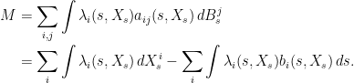
Although this idea is simple enough, there are technical problems to be overcome. To construct the Girsanov transformation, we first define the local martingales

$\displaystyle \setlength\arraycolsep{2pt} \begin{array}{rl} &\displaystyle M=\sum_{j=1}^m \int c_j(s,X_s)\,dB^j_s,\smallskip\\ &U=\mathcal{E}(M)\equiv\exp\left(M-\frac12[M]\right). \end{array}$

(10)

If U is a uniformly integrable martingale then ${{\mathbb Q}=U_\infty\cdot{\mathbb P}}$ would have the required property. Unfortunately, this condition is not satisfied in many cases. Consider, for example, the simple case where ${m=1}$ and c is a nonzero constant. Then, B is a 1-dimensional Brownian motion and is recurrent (hits every value at arbitrarily large times) with probability 1. However, under the transformed measure ${{\mathbb Q}}$ , B will be a Brownian motion plus a constant nonzero drift, and tends to plus or minus infinity with probability one, hence is not recurrent. So, the desired measure ${{\mathbb Q}}$ cannot be equivalent to ${{\mathbb P}}$ .

The solution is to construct ${{\mathbb Q}}$ locally. That is, for each time ${T\ge 0}$ , construct a measure ${{\mathbb Q}_T}$ such that (8) holds over the interval [0,T]. By Novikov’s criterion, the stopped process ${U^T}$ is a uniformly integrable martingale (equivalently, U is a martingale). Indeed, ${[M]_T=\sum_j\int_0^Tc_j(s,X_s)^2\,ds}$ is bounded, so ${\exp(\frac12[M]_T)}$ is integrable. Then, define the measure ${{\mathbb Q}_T}$ on ${(\Omega,\mathcal{F}_T)}$ by ${{\mathbb Q}_T=U_T\cdot {\mathbb P}\vert_{\mathcal{F}_T}}$ .

Note that if ${A\in\mathcal{F}_S}$ and ${S<T}$ then, applying the martingale property for U,

$\displaystyle {\mathbb Q}_S(A)={\mathbb E}[1_AU_S]={\mathbb E}[1_AU_T]={\mathbb Q}_T(A).$

So, ${{\mathbb Q}_S={\mathbb Q}_T\vert_{\mathcal{F}_S}}$ . We would like to imply the existence of a measure ${{\mathbb Q}}$ satisfying ${{\mathbb Q}\vert_{\mathcal{F}_T}={\mathbb Q}_T}$ for all times ${T\ge 0}$ . For such a result to hold, it is necessary to restrict consideration to certain special filtered probability spaces so that Kolmogorov’s extension theorem can be used.

Lemma 3 For some ${d\in{\mathbb N}}$ , let ${\Omega=C({\mathbb R}_+,{\mathbb R}^d)}$ be the space of continuous functions from ${{\mathbb R}_+}$ to ${{\mathbb R}^d}$ , and let Y be the coordinate process,

$\displaystyle \setlength\arraycolsep{2pt} \begin{array}{rl} &\displaystyle Y_t\colon\Omega\rightarrow{\mathbb R}^d,\smallskip\\ &\displaystyle Y_t(\omega)=\omega(t) \end{array}$

( ${t\ge 0}$ ). Furthermore, let ${\mathcal{F}^0_t}$ be the sigma algebra on ${\Omega}$ generated by ${\{Y_s\colon s\le t\}}$ and set ${\mathcal{F}^0=\mathcal{F}^0_\infty}$ .

Suppose that, for each ${T\in{\mathbb R}_+}$ , ${{\mathbb Q}_T}$ is a probability measure on ${(\Omega,\mathcal{F}^0_T)}$ and that ${{\mathbb Q}_S={\mathbb Q}_T\vert_{\mathcal{F}^0_S}}$ whenever ${S\le T}$ . Then, there is a unique measure ${{\mathbb Q}}$ on ${(\Omega,\mathcal{F}^0)}$ satisfying ${{\mathbb Q}\vert_{\mathcal{F}^0_T}={\mathbb Q}_T}$ for all T.

The superscript 0 is used here to signify that the filtration ${\mathcal{F}^0_t}$ is not complete. That is, we do not add all zero probability sets of ${\mathcal{F}^0}$ to the filtration (no probability measure has been defined yet, so this wouldn’t even make any sense). This means that care should be taken when applying results from stochastic calculus, as completeness is often assumed. However, it is only really needed to guarantee cadlag versions of martingales and stochastic integrals, which we do not need to be too concerned about for the moment.

Proof: Let ${\Omega^\prime\supset\Omega}$ be the space of all functions ${{\mathbb R}_+\rightarrow{\mathbb R}^d}$ , with coordinate process ${Y^\prime_t(\omega)=\omega(t)}$ and filtration ${\mathcal{F}^\prime_t=\sigma(Y^\prime_s\colon s\le t)}$ . Under the inclusion ${\Omega\rightarrow\Omega^\prime}$ , ${{\mathbb Q}_T}$ induces a measure ${{\mathbb Q}^\prime_T}$ on ${(\Omega^\prime,\mathcal{F}^\prime_T)}$ . Since ${{\mathbb Q}^\prime_S={\mathbb Q}^\prime_T\vert_{\mathcal{F}^\prime_S}}$ for all ${S\le T}$ , these measures are consistent. So, Kolmogorov’s extension theorem says that there exists a measure ${{\mathbb Q}^\prime}$ on ${(\Omega^\prime,\mathcal{F}^\prime_\infty)}$ such that ${{\mathbb Q}^\prime\vert_{\mathcal{F}^\prime_T}={\mathbb Q}^\prime_T}$ . By construction, ${Y^\prime}$ has a continuous modification over the bounded intervals ${[0,T]}$ so, taking the limit ${T\rightarrow\infty}$ , ${Y^\prime}$ has a continuous modification, ${\tilde Y^\prime}$ on ${{\mathbb R}_+}$ . This defines a measurable map ${\Omega^\prime \rightarrow \Omega}$ , inducing the required measure ${{\mathbb Q}}$ on ${(\Omega,\mathcal{F}^0)}$ . By definition, ${{\mathbb Q}}$ is uniquely determined on the algebra ${\bigcup_T\mathcal{F}^0_T}$ generating ${\mathcal{F}^0}$ so, by the monotone class theorem, this uniquely determines ${{\mathbb Q}}$ . ⬜

We can always restrict consideration to spaces of continuous functions when looking for weak solutions of SDEs.

Lemma 4 Suppose that (7) has a weak solution. Then, there exists a weak solution, with the same initial distribution, on the filtration ${\{\mathcal{F}^0_t\}_{t\ge 0}}$ defined by Lemma 3.

Proof: Let ${X}$ be a weak solution defined on some filtered probability space ${(\tilde\Omega,\mathcal{\tilde F},\{\mathcal{\tilde F}_t\}_{t\ge0},\tilde{\mathbb P})}$ , with respect to the continuous m-dimensional Brownian motion B. Then, ${Z\equiv({\it B},{\it X})}$ is a continuous (m+n)-dimensional process. Taking d=m+n, and letting ${\Omega}$ be as in Lemma 3, Z defines a map from ${\tilde\Omega}$ to ${\Omega}$ and we can define ${{\mathbb P}}$ to be the induced measure ${{\mathbb P}(A)=\tilde{\mathbb P}(Z^{-1}(A))}$ on ${(\Omega,\mathcal{F}^0)}$ . The coordinate process of ${\Omega}$ can be written as ${(B^\prime,X^\prime)}$ , where ${B^\prime\circ Z=B}$ and ${X^\prime\circ Z=X}$ . So, ${(B^\prime,X^\prime)}$ has the same joint distribution as ${(B,X)}$ and ${X^\prime}$ is a weak solution to the SDE with respect to the Brownian motion ${B^\prime}$ . ⬜

Putting this together enable us to apply the required Girsanov transformation locally, transforming the drift of our SDE.

Lemma 5 Let ${X}$ be a weak solution to the SDE (7) for an m-dimensional Brownian motion B, and defined on the filtered probability space ${(\Omega,\mathcal{F}^0,\{\mathcal{F}^0_t\}_{t\ge0},{\mathbb P})}$ , where ${\Omega,\mathcal{F}^0,\mathcal{F}^0_t}$ are as in Lemma 3. For bounded measurable functions ${c_j\colon{\mathbb R}_+\times{\mathbb R}^n\rightarrow{\mathbb R}}$ , let U be the martingale defined by (10).

Then, there is a unique probability measure ${{\mathbb Q}}$ on ${(\Omega,\mathcal{F}^0)}$ such that ${{\mathbb Q}\vert_{\mathcal{F}^0_T}=U_T\cdot{\mathbb P}\vert_{\mathcal{F}^0_T}}$ for each ${T\in{\mathbb R}_+}$ . The process ${\tilde B}$ defined by (8) is a ${{\mathbb Q}}$ -Brownian motion and X is a solution to the SDE (9).

Proof: As shown above, U is a martingale and the measures ${{\mathbb Q}_T=U_T\cdot{\mathbb P}\vert_{\mathcal{F}^0_T}}$ satisfy the condition ${{\mathbb Q}_T\vert_{\mathcal{F}_S}={\mathbb Q}_S}$ for ${S\le T}$ . So, Lemma 4 gives a unique measure ${{\mathbb Q}}$ such that ${{\mathbb Q}\vert_{\mathcal{F}^0_T}={\mathbb Q}_T}$ as required.

Next, by the theory of Girsanov transformations, the stopped processes ${\tilde B^T}$ are ${{\mathbb Q}_T}$ -local martingales, so ${\tilde B}$ is a ${{\mathbb Q}}$ -local martingale. Furthermore, as ${{\mathbb Q}}$ is equivalent to ${{\mathbb P}}$ over finite time horizons, the covariations ${[\tilde B^i,\tilde B^j]=[B^i,B^j]}$ agree under the ${{\mathbb P}}$ and ${{\mathbb Q}}$ measures so, by Lévy’s characterization, ${\tilde B}$ is a ${{\mathbb Q}}$ -Brownian motion. Finally, the SDE (9) follows from substituting expression (8) for ${\tilde B}$ into (7). ⬜

We can now prove weak existence and uniqueness in law for SDEs with transformed drift term.

Theorem 6 Let ${a_{ij},b_i,c_j\colon{\mathbb R}_+\times{\mathbb R}^n\rightarrow{\mathbb R}}$ be measurable functions (i=1,…,n, j=1,…,m) such that ${c_j}$ are bounded. Setting ${\tilde b_i=b_i+\sum_{j=1}^ma_{ij}b_j}$ , consider the SDE

$\displaystyle dX^i_t = \sum_{j=1}^m a_{ij}(t,X_t)\,dB^j_t+\tilde b_i(t,X_t)\,dt.$ (11)

Then,

(11) has a weak solution for any given initial distribution ${\mu}$ for ${X_0}$ if and only if (7) does.
(11) satisfies uniqueness in law for any given initial distribution ${\mu}$ for ${X_0}$ if and only if (7) does.

Proof: By Lemma 4, it is only necessary to use the space ${\Omega=C({\mathbb R}_+,R^d)}$ and filtration ${\mathcal{F}^0_t}$ defined in Lemma 3 when considering weak solutions to the SDE.

Suppose that X is a weak solution to (7) with respect to an m-dimensional Brownian motion B under probability measure ${{\mathbb P}}$ . Then, the transformed measure ${{\mathbb Q}}$ defined by Lemma 5 makes ${\tilde B=B-\int c(s,X_s)\,ds}$ into a Brownian motion, with respect to which X satisfies (7). Therefore, under ${{\mathbb Q}}$ , X is a weak solution to (11). Also, ${{\mathbb Q}\vert_{\mathcal{F}^0_0}={\mathbb P}\vert_{\mathcal{F}^0_0}}$ so X has the same initial distribution under ${{\mathbb P}}$ and ${{\mathbb Q}}$ . This shows that weak existence for (7) implies weak existence for (11). The converse statement follows by exchanging the roles of ${b_i}$ and ${\tilde b_i}$ , and replacing ${c_j}$ by ${-c_j}$ .

Now suppose that (11) satisfies uniqueness in law for solutions with initial distribution ${\mu}$ , and let X be a weak solution to (7) with ${X_0\sim\mu}$ , with respect to m-dimensional Brownian motion B under a measure ${{\mathbb P}}$ . As above, X is a weak solution to (11) under the transformed measure ${{\mathbb Q}}$ with the same initial distribution as under ${{\mathbb P}}$ . So, by uniqueness in law, the distribution of X under ${{\mathbb Q}}$ is uniquely determined. Also, ${c_j}$ can be replaced by ${c_j+c^\prime_j}$ for bounded measurable functions 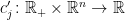${c^\prime_j\colon{\mathbb R}_+\times{\mathbb R}^n\rightarrow{\mathbb R}}$ satisfying ${\sum_ja_{ij}c^\prime_j=0}$ without affecting the conclusion of the theorem. So, by orthogonal projection onto the row-space of ${a_{ij}}$ , we can suppose that ${c_j=\sum_i\lambda_ia_{ij}}$ for some ${\lambda_i}$ . Furthermore, it is not hard to see that ${\lambda_i}$ can be constructed as a measurable function from ${{\mathbb R}_+\times{\mathbb R}^n}$ . So, the local martingale M defined by (10) can be written as

$\displaystyle \setlength\arraycolsep{2pt} \begin{array}{rl} \displaystyle M &\displaystyle= \sum_{i,j}\int\lambda_i(s,X_s)a_{ij}(s,X_s)\,dB^j_s\smallskip\\ &\displaystyle=\sum_i\int\lambda_i(s,X_s)\,dX^i_s-\sum_i\int\lambda_i(s,X_s)b_i(s,X_s)\,ds. \end{array}$

This expresses M, and hence U, entirely in terms of the process X under measure ${{\mathbb Q}}$ , which is uniquely determined due to uniqueness in law of (11). This uniquely defines the measure ${{\mathbb P}}$ , since

$\displaystyle {\mathbb P}(A)={\mathbb E}[1_AU_T^{-1}]$

for all ${T\in{\mathbb R}_+}$ and ${A\in\mathcal{F}^0_T}$ . So, (7) also satisfies uniqueness in law for the given initial distribution of X. The converse statement follows by exchanging the roles of ${b_i}$ and ${\tilde b_i}$ and replacing ${c_j}$ by ${-c_j}$ . ⬜

Finally, this result allows us to prove weak existence and uniqueness in law for the SDE mentioned at the top of the post.

Theorem 7 Let ${a\colon{\mathbb R}\rightarrow{\mathbb R}}$ and ${b\colon{\mathbb R}_+\times{\mathbb R}\rightarrow{\mathbb R}}$ be measurable functions such that a is nonzero, ${a^{-2}}$ is locally integrable and ${b(t,x)/a(x)}$ is bounded. Then, the SDE

$\displaystyle dX_t = a(X_t)\,dB_t+b(t,X_t)\,dt$ (12)

(for Brownian motion B) has weak solutions satisying uniqueness in law.

Proof: Theorem 2 guarantees weak existence and uniqueness in law for the SDE (3) with zero drift term. Then, ${c(t,x)=b(t,x)/a(x)}$ is bounded and measurable, so Theorem 6 extends this to give weak existence and uniqueness in law for SDE (12) with drift ${b=ac}$ . ⬜

Published by George Lowther

View all posts by George Lowther

Published 17 May 1028 October 19

29 thoughts on “SDEs Under Changes of Time and Measure”

Anonymous says:

5 June 10 at 3:04 PM

Change of time.
Consider the SDE $dX(t)=dW(t)$ . A solution of this is $X(t)=X(0)+\sqrt{g} W(\frac{t}{g})$
1) Is the above statement correct?
2) How do we use this fact to solve another problem, such as this:

$\displaystyle dX(t)=a(t,X)dW(t)$

where, perhaps $a(t,X)=\sigma X(t)$ .

Reply
1. George Lowther says:
  
  5 June 10 at 5:35 PM
  
  Hi
  1) It is correct as long as you mean “weak solution”. X will satisfy the SDE $dX=d\tilde W$ where $\tilde W_t$ is the time-changed Brownian motion $\sqrt{g}W_{\frac{t}{g}}$ .
  2) To solve $dX_t=a(t,X_t)\,dW_t$ you need to use a random time-change. If $a(t,X)$ is independent of t, then a weak solution is given by equation (4) in my post. That is, $X_t=X_0+W_{A_t}$ where
  
  $\displaystyle\int_0^{A_t}a(X_0+W_s)^{-2}\,ds=t.$
  
  If $a$ also depends on time then it is more difficult and the time-change technique does not work as well. You can go through the same steps as in my post and, instead of (4), you get the following
  
  $\displaystyle \int_0^ta(s,X_0+W_{A_s})^{-2}\,dA_s=t.$
  
  I changed variables in the post to solve for $A_t$ in (4), but it doesn’t work here because of the dependency on s inside the integral. In differential form
  
  $\displaystyle dA_t=a(t,X_0+W_{A_t})^2\,dt.$
  
  This replaces the SDE by an ODE, but it doesn’t have an explicit solution. Whether solutions exist and are unique is also unclear.
  
  Reply
2. George Lowther says:
  
  5 June 10 at 6:01 PM
  
  Sorry, missed your last line “where perhaps $a(t,X)=\sigma X_t$ “. In this case, $a$ is independent of $t$ , so the method described in my post solves it.
  
  Reply
Anonymous says:

6 June 10 at 4:34 AM

Thank you for your quick reply. Also I am unclear about how to post LaTex so that it looks nice.
Anyway perhaps you can help me as I am struggling a little with this.
Consider the SDE

$\displaystyle dX(t)=\sigma X(t) dB(t)$

So in the notation given in the text, we have

$\displaystyle a(t,X(t))=\sigma X(t)$

Can you please elaborate on the next step? (Again I thank you very much.)

Reply
1. George Lowther says:
  
  7 June 10 at 12:56 AM
  
  To post latex in a comment, use $latex … $ (must include the space after “latex”), and put regular latex between these tags. For “display mode” maths, use the latex keyword \displaystyle and, to center the equation, put between <p align="center"> … </p> html tags. I edited the maths in your posts.
  
  Reply
Anonymous says:

6 June 10 at 4:47 AM

So it seems that the next step is to say

$\displaystyle \int_{0}^{A_t }a(X(0)+B(s))^{-2}ds=t$

which in this example is

$\displaystyle \int_{0}^{A_t }\frac{1}{(\sigma X(0)+\sigma B(s))^2 }ds=t$

…and how on earth do we approach this integral?

Reply
1. George Lowther says:
  
  7 June 10 at 1:08 AM
  
  It is unnecessary to use time changes for the specific case of $dX=\sigma X\,dB$ . This can be solved exactly, using Ito’s lemma. Just rewrite the SDE in terms of $\log X$ , $d\log X_t= \sigma\,dB_t-\frac12\sigma^2dt$ . The solution is the well-known formula for geometric Brownian motion, $X_t = X_0\exp( \sigma B_t-\frac12\sigma^2t)$ .
  
  The time change method is best suited to cases where there is no such exact formula, and its strength lies in generating (weakly) unique solutions even for non-continuous diffusion coefficients. Solving the integral
  
  $\displaystyle \int_{0}^{A_t }\frac{1}{(\sigma X(0)+\sigma B(s))^2 }ds=t$
  
  cannot be done analytically. We know that it does have a unique solution — $A_t$ is just the unique time at which the integral on the LHS hits t. You can’t write it in any significantly simpler form.
  
  Reply
Anonymous says:

7 June 10 at 3:48 AM

Ok, let’s try a different example. Consider the Arithmetic Brownian Motion SDE. I realize this is also probably unnecessarily approached in this way, but I’d like to make sure I understand this.

$\displaystyle dX(t)=\sigma dB(t)$

Then we have

$\displaystyle \int_{0}^{A_t }a(X(0)+W(s))^{-2}ds=t$

which in this case is just

$\displaystyle \int_{0}^{A_t }\frac{1}{\sigma^2 }ds=t$

or

$\displaystyle A_t=\sigma ^2t$

So we have

$\displaystyle A_t=\sigma ^2t$

Is this the correct approach?

Reply
Anonymous says:

7 June 10 at 3:52 AM

Oops sorry about the formatting. ([George]: Fixed, formatting should be fine now) So from above we have

$X(t) = X(0)+W(\sigma^2t)$

This makes sense to me. Do you think I have the right idea?

Reply
1. George Lowther says:
  
  7 June 10 at 9:29 PM
  
  Yes! That all looks right!
  
  Reply
Anonymous says:

7 June 10 at 4:46 AM

Now let’s try the following:

$\displaystyle dX(t)=\sigma e^{\alpha t}dB(t)$

and

$\displaystyle \int_{0}^{A_t}a(X(0)+W(s))^{-2}ds=t$

means

$\displaystyle \int_{0}^{A_t}\frac{1}{\sigma^2 e^{2 \alpha s} } ds=t$

which is

$\displaystyle \frac{(1-e^{-2\alpha A_t} )}{2\alpha \sigma^2}=t$

and hence

$\displaystyle A_t=\frac{Log(1-2\alpha\sigma^2 t)}{-2\alpha}$

so we obtain

$\displaystyle X(t)=X(0)+W(\frac{Log(1-2\alpha\sigma^2 t)}{-2\alpha})$

Does this seem right?

Reply
1. George Lowther says:
  
  7 June 10 at 9:52 PM
  
  No, there is a mistake here. The formulas work out a bit differently from in my post, because you now have time dependent coefficients. The formula I used to derive (4) is $\int_0^ta(s,X_s)^{-2}\,d[X]_s=t$ . Substitute in $A_t=[X]_t$ and $X_t=X_0+W_{A_t}$ ,
  
  $\displaystyle \int_0^t a(s,X_0+W_{A_s})^{-2}\,dA_s = t.$
  
  To arrive at (4) I substituted $A_t$ for t and used the substitution $u=latex A_s$ in the integral. This worked fine when $a$ is time-independent, because $A_s$ appears in the integral, but never s on its own. Now, including the time dependency gives
  
  $\displaystyle \int_0^{A_t} a\left(A^{-1}(u),X_0+W_u\right)^{-2}\,du = t.$
  
  The $A^{-1}(u)$ term messes this up a bit. It’s easiest not to do the substitution and instead use
  
  $\displaystyle A_t=\int_0^ta(s,X_0+W_{A_s})^2\,ds.$
  
  This has A on both sides so it doesn’t give us an explicit solution in general. However, in your case, $a(t,x)=\sigma e^{\alpha t}$ works out fine.
  
  $\displaystyle A_t=\int_0^t\sigma^2e^{2\alpha s}\,ds = \frac{\sigma^2}{2\alpha}(e^{2\alpha s}-1)$
  
  giving,
  
  $\displaystyle X_t=X_0+W\left(\frac{\sigma^2}{2\alpha}(e^{2\alpha t}-1)\right).$
  
  Reply
Anonymous says:

8 June 10 at 5:16 AM

I see, this solution matches what we know about Ornstein-Uhlenbeck vis-a-vis Ito.
I’m grateful for your help. You’ve been very generous with your knowledge – and also forgiving about the LaTex / formatting issues!!
Thanks a million.

Reply
1. George Lowther says:
  
  8 June 10 at 1:08 PM
  
  No problem!
  
  Reply
Anonymous says:

27 July 10 at 11:22 AM

hi, George

The approach in this page is very interesting.
Would you give a reference, which book/article it is based?
Thank you.

Reply
1. George Lowther says:
  
  27 July 10 at 6:42 PM
  
  This post is applying fairly standard techniques that I have seen in several places. I’m not at home to look this up right now, but I’m pretty sure that both the books by Revuz-Yor and Rogers-Williams use the time change method for 1 dimensional diffusions, and also the measure change method (in arbitrary dimensions). The measure change was also used by Stroock-Varadhan to quickly reduce their well known uniqueness result to one without drift.
  
  Reply
  1. Anonymous says:
    
    28 July 10 at 1:29 AM
    
    Thank you very much for several references.
    
    Reply
Anonymous says:

27 July 10 at 4:23 PM

Dear George:

In the proof of Theorem 2, Why is $\int_0^t a(M_s)^{-2} ds < \infty$ almost surely, provided that $a^{-2} \in L^1_{loc}$ ? Thank you.

Reply
1. Anonymous says:
  
  27 July 10 at 4:32 PM
  
  I just find an answer to myself, please verify:
  If $g$ is continuous, then $g\in L^1_{loc}$ , and $L^1_{loc}$ is closed under composition. Hence, because $f, g=M \in L^1_{loc}$ , $f\circ g \in L^1_{loc}$ .
  
  Reply
  1. George Lowther says:
    
    27 July 10 at 6:33 PM
    
    No, that’s not correct, $L^1_{\rm loc}$ is not closed under composition. Theorem 2 only works because M is a semimartingale with quadratic variation $d[M]_t=dt$ , and then equation (6) is applied.
    
    Reply
Anonymous says:

28 July 10 at 1:55 AM

Dear George,

Here is my understanding:
$f\in L^1_{loc}$ is required to have $F(x)$ is well defined.
So, Ito identity (6) makes sense, and it implies all terms in (6) are a.s. finite.
Thank you very much.

Reply
Ivan Dornic says:

11 January 11 at 11:30 AM

Hi George,

First congrats for this very nice blog, where things in the literature are made edible for somebody not trained in a pure probability playground (I am a physicist…).

In the SDE (3), $dX_t = a(X_t)dB_t$ , I was wondering how crucial is the condition you mention that $a$ is never zero. What I have in mind is the so-called Kimura’s diffusion where $a(X)=\sqrt{1-X^2}$ : the state space is the interval $I=[-1,1]$ (starting from $X_0=x_0$ within it), and it is known that that the solution hits either ±1 in a finite mean time and stays there forever.
Related question related to a possible time-change: set $X_t=\sin{\theta_t}$ , with $\theta_t \in (-\pi/2,\pi/2)$ . Then by Itô’s formula

$\displaystyle d \theta_t = 1/(2 \cos{\theta_t}) + dB_t$

Does there exist a change of time $\tau_t$ which allows to rewrite
$\theta_t= B_{\tau_t}$ ?
How is this useful to say recover the known expression for the conditional transition
probability distribution function ${\rm Proba}[X_t=x|X_0=x_0]$ ?

Best,

Ivan Dornic

Reply
1. George Lowther says:
  
  13 January 11 at 2:12 AM
  
  Hi Ivan,
  
  Thanks for your comment. I assumed that $a$ is never zero for simplicity here. The aim of this post was really to demonstrate the techniques of time and measure changes rather than give as general as possible a statement on the solutions to SDEs.
  
  Anyway, if $a$ does hit zero, then there are several possibilities for the SDE $dX=a(X)\,dB$ , which can also be handled by the time change method.
  
  i) $a(x_0)=0$ for some value of x₀, but $a^{-2}$ is still locally integrable (so that $a$ can only vanish on a set of measure zero). In this case, there exist solutions to the SDE, but they are not unique. For example, consider $dX=1_{\{X\not=0\}}\,dB$ . Then $X=B$ satisfies this. However, letting X equal B but stopped at some time when it hits zero will give another solution. If you require that the set $\{t\colon X_t=0\}$ has zero lebesgue measure, then the solution is unique.
  
  ii) $\int_{x_0-\epsilon}^{x_0}a(x)^{-2}\,dx$ and $\int_{x_0}^{x_0+\epsilon}a(x)^{-2}\,dx$ are both infinite. In this case there is a unique solution, but the boundary is not accessible (unless you start the process at the boundary, in which case it stays there).
  
  iii) $\int_{x_0-\epsilon}^{x_0}a(x)^{-2}\,dx$ is finite but $\int_{x_0}^{x_0+\epsilon}a(x)^{-2}\,dx$ is infinite. Here, we still have uniqueness in law. In this case the boundary is accessible from below (but not above), and is absorbing. This is the case for the upper boundary $x_0=1$ in your example.
  
  iv) As with (iii), but where the boundary is accessible from above.
  
  These situations are handled by the time change method. For example, consider my expression (4) in the post, in case (iii). As the Brownian motion $X_0+W_t$ approaches $x_0$ from above at some time $\tau$ , the integral of $a(X_0+W_t)^{-2}$ diverges so, inverting this, $A_t$ approaches $\tau$ but never reaches it. This implies that the processes $X$ approaches $x_0$ from above, but never reaches it in finite time. On the other hand, as $X_0+W_t$ approaches $x_0$ from below the integral of $a(X_0+W_t)^{-2}$ is bounded, but diverges immediately after $\tau$ . So, $A$ approaches time $\tau$ in finite time, then jumps to infinity. Applying the time change, the solution $X_t$ hits $x_0$ and stays there.
  
  In your example, $dX = \sqrt{1-X^2}\,dB$ , the process can hit either 1 or -1 in finite time, and always will hit one of these as, under the time change, it is just a Brownian motion which will hit -1 or 1.
  
  [btw, I edited the latex in your post].
  
  Reply
2. George Lowther says:
  
  13 January 11 at 2:20 AM
  
  And, for your second question. You can time-change X to a Brownian motion (stopped when it hits ±1) because it is a continuous local martingale. However, theta is not. Your displayed expression shows that it has a drift term $\sin\theta_t dt/(2\cos\theta_t)$ (I think you have a typo in your formula?). You could transform it to a Brownian motion stopped at ±π/2 by a measure change to remove the drift – that is, a Girsanov transform as discussed in this post. I’m not sure how well it works out for explicitly computing the conditional probabilities though. You will get an expectation of an exponential term involving the drift term, which is probably rather messy (but I haven’t tried). Adding a constant drift via Girsanov transforms is easy though and is one way to compute the probability of BM with drift hitting a barrier.
  
  Hope that helps!
  
  Reply
stochasticeduc says:

6 May 13 at 8:56 PM

i have some various question

so first how we can get this :
$$
e^{bt} \ \int_0^t \ f(s) ds=\int_0^t \ ( e^{-bs} \ f(s)-be^{-bs}\int_0^s\ f(u)\ du) \ ds
$$

i need explanation in details please

Second question if we have stopping time and X is stochastic processus in Rn
$$
T=inf ( { t>=0 , X_{s \wedge T}^2 + Y _{s \wedge T}^2 >= A }) \ \ or \\
T=inf ( { t>=0 , | X_t | \geq A + | Y _t | \geq A } )
$$ so how we can prove that :
$$
\ {E}(| X _{s \wedge T} – Y _{s \wedge T} |^2) \leq \propto
$$
is finite

The third question how we can get that :

$$-\int_0^t \ sgn(X_{s}) \ dB_{s}=\int_0^t \ sgn(-X_{s})\ dB_{s}+2\int_0^t 1_{X_{s} =0}dB_{s}$$
with B is brownian motion on Rn ,and sgn is Sign function

i took this from Tanaka ‘s SDE to prove that there ‘s non pathwise uniquenss

so please if you have examle of SDE that has strong solution without strong uniquenss (pathwise uniquenss)

Thanks for Your time
i’ll be grateful for ur help

best,
Educ

Reply
TheBridge says:

22 May 21 at 5:57 PM

Hi There is a little typo in theorem 6 where it should be c_i and not b_i regards

Reply
1. TheBridge says:
  
  23 May 21 at 8:21 AM
  
  To be more precise I meant c_i.a_{ij} instead of b_i.a_{ij} in the seting of \tilda[b_i}
  
  Reply
leejulian6702 says:

15 March 22 at 7:44 PM

Hi George, again I have several questions regarding the details of the proofs. I would greatly appreciate if you could help me understand them.

1. In the proof of Theorem 2, how does the identity for F(M_t) extends to nonnegative locally integrable functions f by monotone convergence? The application of the monotone class theorem part seems to follow from the fact that continuous functions approximate bounded measurable functions and monotone class theorem involves bounded monotone limits, so dominated convergence theorems for Lebesgue Stieltjes integral and stochastic integrals apply on all terms of the identity.
However, I am not aware of any approximation results for locally integrable functions via bounded measurable functions. To use monotone convergence, as F itself is defined in terms of Lebesgue integral and we have a stochastic integral and L-S integral on the Right hand side terms, we would need to use dominated or bounded convergence theorems on the RHS and on the LHS to extend the identity.
Moreover, I do not know why f being locally integrable would give the integrability of \int_0^t F'(M)dM and \int_0^t f(M)d[M] in the first place.

2. In the proof of Lemma 3, I think you are taking Y’ to be the image of Y under the inclusion map defined from the continuous function space. And extend Y’ to [0,\infty) from [0,T]. But how does this define a map from all of \Omega’, which is just the space of all functions R_+ \to R^d to C(R_+,R^d)? I don’t understand how we get a continuous modification for every function R_+ \to R^d from the construction here. And why does this map become measurable?

3. In the proof of Lemma 4, my understanding is that B’ is the projection map onto the first R^m and X’ is the projection map onto the next R^n space. Then I can see that (B’,X’) ~ (B,X) in distribution, but why does the equivalence of joint distributions and the fact that X is a weak solution imply that X’ is also a weak solution with respect to the Brownian motion B’?

4. Finally, in the proof of Theorem 6, could you explain the sentence “So, by orthogonal projection onto the row-space of a_ij, we can suppose that c_j = \sum_i \lambda_i a_ij for some \lambda_i”? I can’t figure out why we are able to choose c to be some orthogonal projection onto the row-space of a. And why is the \lambda_i constructed this way measurable?

Thank you

Reply
nasser nasir says:

31 December 22 at 10:03 PM

Hi
who can solve the equation dxt=(Q1- Q2 ) xt dt+ Q3 dwt by using change measure

Reply

	Harry on Filtrations and Adapted P…
	Anonymous on Analytic Sets
	Daniel on Analytic Sets
	Sid on Martingale Convergence
	northwiz on Preservation of the Local Mart…
	George Lowther on Martingale Convergence
	Sid on Martingale Convergence
	George Lowther on The Burkholder-Davis-Gundy Ine…
	George Lowther on Preservation of the Local Mart…
	northwiz on Preservation of the Local Mart…

Changes of Time

Changes of Measure

Like this:

Related

Published by George Lowther

29 thoughts on “SDEs Under Changes of Time and Measure”

Leave a Reply Cancel reply