Stochastic differential equations (SDEs) form a large and very important part of the theory of stochastic calculus. Much like ordinary differential equations (ODEs), they describe the behaviour of a dynamical system over infinitesimal time increments, and their solutions show how the system evolves over time. The difference with SDEs is that they include a source of random noise., typically given by a Brownian motion. Since Brownian motion has many pathological properties, such as being everywhere nondifferentiable, classical differential techniques are not well equipped to handle such equations. Standard results regarding the existence and uniqueness of solutions to ODEs do not apply in the stochastic case, and cannot readily describe what it even means to solve such as system. I will make some posts explaining how the theory of stochastic calculus applies to systems described by an SDE.
Consider a stochastic differential equation describing the evolution of a real-valued process {Xt}t≥0,
 |
(1) |
which can be specified along with an initial condition X0 = x0. Here, b is the drift specifying how X moves on average across the dt time, σ is a volatility term giving the amplitude of the random noise and W is a driving Brownian motion providing the source of the randomness. There are numerous situations where equations such as (1) are used, with applications in physics, finance, filtering theory, and many other areas.
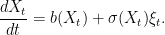
In the case where σ is zero, (1) is just an ordinary differential equation dX/dt = b(X). In the general case, we can informally think of dividing through by dt to give an ODE plus an additional noise term
 |
(2) |
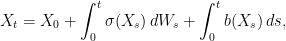
I have set ξt = dWt/dt which can be thought of as a process whose values at each time are independent zero-mean random variables. As mentioned above, though, Brownian motion is not differentiable so this does not exist in the usual sense. While it can be described by a kind of random distribution, even distribution theory is not well-equipped to handle such equations involving multiplying by the nondifferentiable process σ(Xt). Instead, (1) can be integrated to obtain
 |
(3) |
where the right-hand-side is interpreted using stochastic integration with respect to the semimartingale W. Likewise, X will be a semimartingale, and such solutions are often referred to as diffusions.
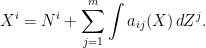
The differential form (1) can be interpreted as a shorthand for the integral expression (3), which I will do in these notes. It can be generalized to n-dimensional processes by allowing b to take values in ℝn, σ(x) to be an n × m matrix, and W to be an m-dimensional Brownian motion. That is, W = (W1, …, Wm) where Wi are independent Brownian motions. I will sometimes write this as
 |
where the summation convention is being applied, with subscripts or superscripts occuring more than once in a single term being summed from 1 to n.
Unlike ODEs, when dealing with SDEs we need to consider what underlying probability space the solution is defined with respect to. This leads to the existence of different classes of solutions.
- Strong solutions where X can be expressed as a measurable function of the Brownian motion W or, equivalently, X is adapted to its natural filtration.
- Weak solutions where X need not be a function of W. Such cases may require additional randomness so may not exist on the probability space with respect to which the Brownian motion W is defined. It can be necessary to extend the filtered probability space to construct these solutions.
Likewise, when considering uniqueness of solutions, there are different ways this occurs.
- Pathwise uniqueness where, up to indistinguishability, there is only one solution X. This should hold not just on one specific space containing a Brownian motion W, but on all such spaces. That is, weak solutions should be unique.
- Uniqueness in law where there may be multiple pathwise solutions, but their distribution is uniquely determined by the SDE.
There are various general conditions under which strong solutions and pathwise uniqueness are guaranteed for SDE (1) , such as the Itô result for Lipschitz continuous coefficients. I covered this situation in a previous post.
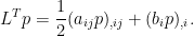
Other than using the SDE (1), such systems can also be described by an associated differential operator. For the n-dimensional case set a(x) = σ(x)σ(x)T, which is an n × n positive semidefinite matrix. Then, the second order operator L can be defined
 |
operating on twice continuously differentiable functions f: ℝn → ℝ. Being able to effortlessly switch between descriptions using the SDE (1) and the operator L is a huge benefit when working with such systems. There are several different ways in which the operator can be used to describe a stochastic process, all of which relate to weak solutions and uniqueness in law of the SDE.
Markov Generator: A Markov process is a weak solution to the SDE (1) if its infinitesimal generator is L. That is, if the transition function is Pt then,
 |
for suitably regular functions f.
Backwards Equation: For a function f: ℝn × ℝ+ → ℝ, f(t, Xt) is a local martingale if and only if it solves the partial differential equation (PDE)
 |
Consequently, for any time t > 0 and function g: ℝd → ℝ, if we let f be a solution to the PDE above with boundary condition f(x, t) = g(x) then, assuming integrability conditions, the conditional expectations at times s < t are
![\displaystyle {\mathbb E}[g(X_t)\;\vert\mathcal F_s]=f(X_s,s).](https://s0.wp.com/latex.php?latex=%5Cdisplaystyle+%7B%5Cmathbb+E%7D%5Bg%28X_t%29%5C%3B%5Cvert%5Cmathcal+F_s%5D%3Df%28X_s%2Cs%29.+&bg=ffffff&fg=000000&s=0&c=20201002) |
If the conditions are satisfied, this describes a Markov process and gives its transition probabilities, describing the distribution of X and implying uniqueness in law.
Forward Equation: Assuming that it is sufficiently smooth, the probability density p(t, x) of Xt satisfies the PDE
 |
where LT is the transpose of operator L
 |
If this PDE has a unique solution for given initial distribution, then this uniquely determines the distribution of Xt. So, if unique solutions to the forward equation exist starting at every future time, it gives uniqueness in law for X.
Martingale problem: Any weak solution to SDE (1) satisfies the property that
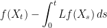 |
is a local martingale for twice continuously differentiable functions f: ℝn → ℝ. This approach, which was pioneered by Stroock and Varadhan, has many benefits over the other applications of operator L described above, since it applies much more generally. We do not need to a-priori impose any properties on X such as being Markov, and as the test functions f are chosen at will, they automatically satisfy the necessary regularity properties. As well as being a very general way to describe solutions to a stochastic dynamical system, it turns out to be very fruitful. The striking and far-reaching Stroock–Varadhan uniqueness theorem, in particular, guarantees existence and uniqueness in law so long as a is continuous and positive definite and b is locally bounded.
 for
for  is related to the fact that, for
  , the process hits zero. This idea extends to all continuous and nonnegative local martingales. The Girsanov transform method applied here is essentially the same as that used by Carlos A. Sin (
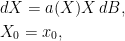
 , B is a Brownian motion and the fixed initial condition
  is strictly positive. The multiplier X in the coefficient of dB ensures that if X ever hits zero then it stays there. By
  is locally integrable on
  . Consider also the following SDE,

![{{\mathbb E}[X_t]=xe^{bt}}](https://s0.wp.com/latex.php?latex=%7B%7B%5Cmathbb+E%7D%5BX_t%5D%3Dxe%5E%7Bbt%7D%7D&bg=ffffff&fg=000000&s=0&c=20201002) , based on the idea that X has growth rate b on average. A more detailed argument is to write out (
, based on the idea that X has growth rate b on average. A more detailed argument is to write out (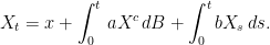
![\displaystyle {\mathbb E}[X_t]=x+\int_0^tb{\mathbb E}[X_s]\,ds.](https://s0.wp.com/latex.php?latex=%5Cdisplaystyle++%7B%5Cmathbb+E%7D%5BX_t%5D%3Dx%2B%5Cint_0%5Etb%7B%5Cmathbb+E%7D%5BX_s%5D%5C%2Cds.+&bg=ffffff&fg=000000&s=0&c=20201002)
![{d{\mathbb E}[X_t]/dt=b{\mathbb E}[X_t]}](https://s0.wp.com/latex.php?latex=%7Bd%7B%5Cmathbb+E%7D%5BX_t%5D%2Fdt%3Db%7B%5Cmathbb+E%7D%5BX_t%5D%7D&bg=ffffff&fg=000000&s=0&c=20201002) , which has the unique solution
, which has the unique solution ![{{\mathbb E}[X_t]={\mathbb E}[X_0]e^{bt}}](https://s0.wp.com/latex.php?latex=%7B%7B%5Cmathbb+E%7D%5BX_t%5D%3D%7B%5Cmathbb+E%7D%5BX_0%5De%5E%7Bbt%7D%7D&bg=ffffff&fg=000000&s=0&c=20201002) .
. there is no problem, and
 ![{{\mathbb E}[X_t]<xe^{bt}}](https://s0.wp.com/latex.php?latex=%7B%7B%5Cmathbb+E%7D%5BX_t%5D%3Cxe%5E%7Bbt%7D%7D&bg=ffffff&fg=000000&s=0&c=20201002) holds.
holds. of dB grows too fast in X.
![\displaystyle {\mathbb E}[X_t\mid\mathcal{F}_s]<X_s](https://s0.wp.com/latex.php?latex=%5Cdisplaystyle++%7B%5Cmathbb+E%7D%5BX_t%5Cmid%5Cmathcal%7BF%7D_s%5D%3CX_s+&bg=ffffff&fg=000000&s=0&c=20201002)
 . Furthermore, for any positive constant
  ,
, ![{{\mathbb E}[X_t^p]}](https://s0.wp.com/latex.php?latex=%7B%7B%5Cmathbb+E%7D%5BX_t%5Ep%5D%7D&bg=ffffff&fg=000000&s=0&c=20201002) is bounded over
is bounded over  and tends to zero as
  .
. and a Brownian motion B


 are fixed real numbers. The function
  has derivative
  which, for
  , is bounded on bounded subsets of the reals. It follows that f is Lipschitz continuous on such bounded sets. However, the derivative of f diverges to infinity as x goes to infinity, so f is not globally Lipschitz continuous. Similarly, if
  then f is Lipschitz continuous on compact subsets of
  , but not globally Lipschitz. To be more widely applicable, the results of the previous post need to be extended to include such locally Lipschitz continuous coefficients.
 , this has the solution
  , which explodes at time
  .
.  in n-dimensional phase space is of the form
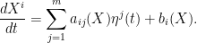
 , and the problem is to find a solution for X, given its value at an initial time. What distinguishes this from an ordinary differential equation are random noise terms
  and, consequently, solutions to the Langevin equation are stochastic processes. It is difficult to say exactly how
  are continuous with independent and identically distributed increments. A candidate for such a process is
  do not have well defined values. Instead, we can rewrite equation (
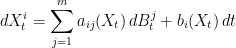
 are independent Brownian motions. This is to be understood in terms of the
  are
are  and time t by arbitrary
  . In integral form, the general SDE for a