Properties of Quasimartingales

The previous two posts introduced the concept of quasimartingales, and noted that they can be considered as a generalization of submartingales and supermartingales. In this post we prove various basic properties of quasimartingales and of the mean variation, extending results of martingale theory to this situation.

We start with a version of optional stopping which applies for quasimartingales. For now, we just consider simple stopping times, which are stopping times taking values in a finite subset of the nonnegative extended reals ${\bar{\mathbb R}_+=[0,\infty]}$ . Stopping a process can only decrease its mean variation (recall the alternative definitions ${{\rm Var}}$ and ${{\rm Var}^*}$ for the mean variation). For example, a process X is a martingale if and only if ${{\rm Var}(X)=0}$ , so in this case the following result says that stopped martingales are martingales.

Lemma 1 Let X be an adapted process and ${\tau}$ be a simple stopping time. Then

$\displaystyle {\rm Var}^*(X^\tau)\le{\rm Var}^*(X).$ (1)

Assuming, furthermore, that X is integrable,

$\displaystyle {\rm Var}(X^\tau)\le{\rm Var}(X).$ (2)

and, more precisely,

$\displaystyle {\rm Var}(X)={\rm Var}(X^\tau)+{\rm Var}(X-X^\tau)$ (3)

Proof: We start by proving (3), and (2) is a simple corollary of this. From lemma 6 of the previous post on quasimartingales, the mean variation can be expressed as

$\displaystyle {\rm Var}(X)=\sup{\mathbb E}\left[\int_0^\infty\xi\,dX\right],$

where the supremum is taken over elementary processes ${\lvert\xi\rvert\le1}$ . Choosing any elementary processes ${\lvert\alpha\rvert\le1}$ and ${\lvert\beta\rvert\le1}$ , set ${\xi=1_{(0,\tau]}\alpha+1_{(\tau,\infty)}\beta}$ . As ${\tau}$ is a simple stopping time, this is elementary and,

$\displaystyle \setlength\arraycolsep{2pt} \begin{array}{rl} &\displaystyle{\mathbb E}\left[\int_0^\infty\alpha\,dX^\tau+\int_0^\infty\beta\,d(X-X^\tau)\right]\smallskip\\ &\displaystyle\qquad= {\mathbb E}\left[\int_0^\infty\xi\,dX\right]\le{\rm Var}(X) \end{array}$

Taking the supremum over all such ${\alpha,\beta}$ ,

$\displaystyle {\rm Var}(X^\tau)+{\rm Var}(X-X^\tau)\le{\rm Var}(X).$

The reverse inequality is just the triangle inequality, so we obtain (3).

Next, to prove (1), we assume that ${{\rm Var}^*(X)}$ is finite, otherwise the result is trivial. Then, X is integrable. Extend X to all times in ${\bar{\mathbb R}_+}$ , by setting ${X_\infty=0}$ . Then, by lemma 10 of the quasimartingale post

$\displaystyle {\rm Var}^*(X)=\sup{\mathbb E}\left[\int_0^\infty\xi\,dX\right].$

The supremum is over all elementary processes ${\lvert\xi\rvert\le1}$ with time index running over ${\bar{\mathbb R}_+}$ . Let us also extend the stopped process ${X^\tau}$ to this index set, by setting ${X^\tau_\infty=0}$ . Then,

$\displaystyle \setlength\arraycolsep{2pt} \begin{array}{rl} \displaystyle{\mathbb E}\left[\int_0^\infty\xi\,dX^\tau\right] &\displaystyle={\mathbb E}\left[\int_0^\infty1_{(0,\tau]}\xi\,dX + \xi_\tau(0-X_\tau)\right] \smallskip\\ &\displaystyle={\mathbb E}\left[\int_0^\infty(1_{(0,\tau]}\xi+\xi_\tau1_{(\tau,\infty]})\,dX\right] \smallskip\\ &\displaystyle\le{\rm Var}^*(X) \end{array}$

as required. ⬜

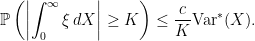
This result can be used to extend Doob’s submartingale inequality to quasimartingales.

Theorem 2 Let X be a cadlag adapted process and K be a nonnegative real. Then,

$\displaystyle {\mathbb P}\left(\sup_{t\ge0}\vert X_t\vert\ge K\right)\le\frac1K{\rm Var}^*(X).$

Proof: For any finite ${T\subseteq {\mathbb R}_+}$ , define the simple stopping time

$\displaystyle \tau=\inf\left\{t\in T\colon\lvert X_t\rvert\ge K\right\}$

Then, ${\tau < \infty}$ and ${\lvert X_\tau\rvert\ge K}$ whenever ${\sup_{t\in T}\lvert X_t\rvert\ge K}$ . So, letting ${t^*=\max T}$ ,

$\displaystyle \setlength\arraycolsep{2pt} \begin{array}{rl} \displaystyle{\mathbb P}\left(\sup_{t\in T}\lvert X_t\rvert\ge K\right)&\displaystyle={\mathbb P}\left(\lvert X^\tau_{t^*}\rvert\ge K\right) \smallskip\\ &\displaystyle\le\frac1K{\mathbb E}\left[\lvert X^\tau_{t^*}\rvert\right] \le\frac1K{\rm Var}^*(X^\tau) \smallskip\\ &\displaystyle\le\frac1K{\rm Var}^*(X) \end{array}$

The final inequality here is an application of lemma 1. Now, let ${T}$ be a countable dense subset of ${{\mathbb R}_+}$ and ${T_n}$ be a sequence of finite subsets of ${{\mathbb R}_+}$ increasing to ${T}$ . By right-continuity, if ${\sup_t\lvert X_t\rvert\ge K}$ then, for any ${K^\prime < K}$ , we have ${\sup_{t\in T_n}\lvert X_t\rvert\ge K^\prime}$ for large ${n}$ . So,

$\displaystyle \setlength\arraycolsep{2pt} \begin{array}{rl} \displaystyle{\mathbb P}\left(\sup_{t\ge0}\lvert X_t\rvert\ge K\right)&\displaystyle\le\liminf_{n\rightarrow\infty}{\mathbb P}\left(\sup_{t\in T_n}\lvert X_t\rvert\ge K^\prime\right) \smallskip\\ &\displaystyle\le\frac1{K^\prime}{\rm Var}^*(X) \end{array}$

Letting ${K^\prime}$ increase to ${K}$ gives the result. ⬜

Next, we look at stochastic integrals with respect to elementary integrands. From the mean variation of a process, it is not possible to give ${L^1}$ -bounds for stochastic integrals with respect to that process, even for uniformly bounded integrands. However, the integrals are bounded in probability. The following generalises Lemma 4 of the post on martingales as integrators. In particular, from the post on existence of stochastic integrals, this implies that quasimartingales are semimartingales, although this fact also follows from Rao’s theorem decomposition and the fact that submartingales are semimartingales.

Lemma 3 There exists a constant ${c > 0}$ such that, for any elementary predictable process ${\lvert\xi\rvert\le1}$ , adapted process X, and ${K > 0}$ ,

$\displaystyle {\mathbb P}\left(\left\lvert\int_0^\infty\xi\,dX\right\rvert\ge K\right)\le\frac{c}K{\rm Var}^*(X).$

Proof: I will prove this by extending Lemma 4 from the post on martingales as integrators, which says that there is a ${c > 0}$ such that

$\displaystyle {\mathbb P}\left(\left\lvert\int_0^t\xi\,dM\right\rvert\ge K\right)\le\frac{c}K{\mathbb E}[\lvert M_t\rvert]$

for any martingale ${M}$ .

We suppose that ${{\rm Var}^*(X)}$ is finite so that X is integrable, otherwise the result is trivial. Now, there exists a sequence of times ${t_0 < t_1 < \cdots < t_n}$ such that

$\displaystyle \xi=\sum_{k=1}^n Z_k1_{(t_{k-1},t_k]}$

where ${\lvert Z_k\rvert\le 1}$ is ${\mathcal{F}_{t_{k-1}}}$ -measurable. Now consider a Doob decomposition

$\displaystyle X_{t_k}=M_k+A_k$

where ${A_k=\sum_{j=1}^k{\mathbb E}[X_{t_j}-X_{t_{j-1}}\;\vert\mathcal{F}_{t_{j-1}}]}$ , and ${M}$ is a martingale restricted to the index set ${0,1,\ldots,n}$ . We write ${Z\cdot A_k}$ for the discrete integral ${\sum_{j=0}^kZ_j(A_j-A_{j-1})}$ . The definition of ${{\rm Var}}$ gives

$\displaystyle {\mathbb P}\left(\left\lvert Z\cdot A_n\right\rvert\ge K\right)\le\frac1K{\mathbb E}\left[\left\lvert Z\cdot A_n\right\rvert\right]\le\frac1K{\rm Var}(X).$

Similarly, we can bound the martingale M in ${L^1}$ ,

$\displaystyle {\mathbb E}[\lvert M_n\rvert]\le{\mathbb E}[\lvert X_{t_n}\rvert +\lvert A_n\rvert]\le{\rm Var}^*(X).$

Hence, as stated above,

$\displaystyle {\mathbb P}\left(\lvert Z\cdot M_n\rvert\ge K\right)\le\frac{c}K{\rm Var}^*(X)$

Combining these inequalities,

$\displaystyle \setlength\arraycolsep{2pt} \begin{array}{rl} \displaystyle{\mathbb P}\left(\left\lvert\int_0^\infty\xi\,dX\right\rvert\ge K\right) &\displaystyle= {\mathbb P}\left(\lvert Z\cdot M_n + Z\cdot A_n\rvert\ge K\right) \smallskip\\ &\displaystyle\le {\mathbb P}\left(\lvert Z\cdot M_n\rvert\ge K/2\right) + {\mathbb P}\left( \lvert Z\cdot A_n\rvert\ge K/2\right) \smallskip\\ &\displaystyle\le \frac{2c}K{\rm Var}^*(X)+\frac2K{\rm Var}(X) \end{array}$

So the result follows by replacing ${2c+2}$ by ${c}$ in the above. ⬜

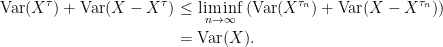
Next, the mean variation behaves as we would expect under ${L^1}$ limits.

Lemma 4 Let ${X^n,X}$ be integrable adapted processes such that ${X^n_t\rightarrow X_t}$ in ${L^1}$ as n goes to infinity. Then,

$\displaystyle \setlength\arraycolsep{2pt} \begin{array}{rl} \displaystyle {\rm Var}(X)&\le\liminf_{n\rightarrow\infty}{\rm Var}(X^n)\smallskip\\ \displaystyle {\rm Var}^*(X)&\le\liminf_{n\rightarrow\infty}{\rm Var}^*(X^n) \end{array}$

Proof: Letting ${\lvert\xi\rvert\le1}$ be an elementary process on time index set ${[0,\infty)}$ , ${L^1}$ convergence gives

$\displaystyle \setlength\arraycolsep{2pt} \begin{array}{rl} \displaystyle{\mathbb E}\left[\int_0^\infty\xi\,dX\right]&\displaystyle=\lim_{n\rightarrow\infty}{\mathbb E}\left[\int_0^\infty\xi\,dX^n\right]\smallskip\\ &\displaystyle\le\liminf_{n\rightarrow\infty}{\rm Var}(X^n). \end{array}$

Taking the supremum over all such ${\xi}$ gives the inequality for ${{\rm Var}(X)}$ . The inequality for ${{\rm Var}^*(X)}$ follows in the same way, except that we set ${X^n_\infty=X_\infty=0}$ and let ${\lvert\xi\rvert\le1}$ range over the elementary processes with time index set ${[0,\infty]}$ . ⬜

The optional stopping result, Lemma 1, can be extended to arbitrary stopping times. The proof will require approximating by simple stopping times and taking limits in ${L^1}$ but, before doing this, we will need to know that such approximations converge in ${L^1}$ . To that end, we extend lemma 6 of the post on cadlag modifications to the quasimartingale case. This requires a filtered probability space ${(\Omega,\mathcal{F},\{\mathcal{F}_t\}_{t\in\mathbb{T}},{\mathbb P})}$ for an arbitrary linearly ordered time index set ${\mathbb{T}}$ . For an integrable process defined on such a space, we define the mean variation as

$\displaystyle {\rm Var}_{\mathbb{T}}(X)=\sup{\mathbb E}\left[\sum_{k=1}^n{\mathbb E}[X_{t_k}-X_{t_{k-1}}\;\vert\mathcal{F}_{t_{k-1}}]\right].$

The supremum is taken over all finite sequences ${t_0\le t_1\le\cdots\le t_n}$ in ${\mathbb{T}}$ . Then, the following lemma holds.

Lemma 5 Let X be an integrable adapted process with respect to a filtered probability space ${(\Omega,\mathcal{F},\{\mathcal{F}_t\}_{t\in\mathbb{T}},{\mathbb P})}$ such that ${{\rm Var}_{\mathbb{T}}(X) < \infty}$ .

Then, ${\{X_{t_n}\}_{n=1,2,\ldots}}$ is uniformly integrable for any decreasing sequence ${t_n\in\mathbb{T}}$ .

Proof: Define the random variable

$\displaystyle A^*=\sum_{k=1}^\infty\left\lvert{\mathbb E}[X_{t_k}-X_{t_{k+1}}\;\vert\mathcal{F}_{t_{k+1}}]\right\rvert$

Monotone convergence shows that this is integrable and, in particular, is almost surely finite

$\displaystyle \setlength\arraycolsep{2pt} \begin{array}{rl} \displaystyle{\mathbb E}[A^*]&\displaystyle=\lim_{n\rightarrow\infty}{\mathbb E}\left[\sum_{k=1}^n\left\lvert{\mathbb E}[X_{t_k}-X_{t_{k+1}}\;\vert\mathcal{F}_{t_{k+1}}]\right\rvert\right] \smallskip\\ &\displaystyle\le{\rm Var}_{\mathbb{T}}(X) \end{array}$

So, the following sum is almost surely convergent, and converges in ${L^1}$

$\displaystyle A_n=\sum_{k=n}^\infty {\mathbb E}[X_{t_k}-X_{t_{k+1}}\vert\mathcal{F}_{t_{k+1}}].$

Furthermore, ${\lvert A_n\rvert\le A^*}$ , so the sequence ${A_n}$ is uniformly integrable. Then, from the definition of ${A_n}$ , the martingale property

$\displaystyle X_{t_n}-A_n={\mathbb E}[X_{t_1}-A_1\;\vert\mathcal{F}_{t_n}]$

is satisfied and the sequence ${X_{t_n}-A_n}$ is uniformly integrable. So, ${X_{t_n}=(X_{t_n}-A_n)+A_n}$ is a uniformly integrable sequence. ⬜

We now extend optional stopping to arbitrary stopping times.

Lemma 6 Let X be a right-continuous adapted process and ${\tau}$ be a stopping time. Then

$\displaystyle {\rm Var}^*(X^\tau)\le{\rm Var}^*(X).$ (4)

Assuming, furthermore, that X is a quasimartingale, then ${X^\tau}$ is integrable and

$\displaystyle {\rm Var}(X^\tau)\le{\rm Var}(X).$ (5)

and, more precisely,

$\displaystyle {\rm Var}(X)={\rm Var}(X^\tau)+{\rm Var}(X-X^\tau).$ (6)

Proof: For the first inequality we can assume without loss of generality that ${{\rm Var}^*(X)}$ is finite, so that X is integrable. So, in either case, we can suppose that X is integrable and ${{\rm Var}(X)}$ is finite.

Now, choose a sequence of simple stopping times ${\tau_n}$ decreasing to ${\tau}$ as n goes to infinity. We show that ${X^{\tau_n}_t\rightarrow X^{\tau}_t}$ in ${L^1}$ , To do this, let ${\mathbb{T}}$ be the negative integers and set ${Y_n=X_{\tau_{-n}\wedge t}}$ and ${\mathcal{G}_n=\mathcal{F}_{\tau_{-n}\wedge t}}$ for each ${n\in\mathbb{T}}$ . We can show that ${{\rm Var}_{\mathbb{T}}(Y)}$ is finite. For any decreasing sequence of positive integers ${n_0\ge n_1\ge\cdots \ge n_k}$ ,

$\displaystyle \setlength\arraycolsep{2pt} \begin{array}{rl} \displaystyle\sum_{j=1}^k\left\lvert{\mathbb E}[Y_{-n_j}-Y_{-n_{j-1}}\;\vert\mathcal{G}_{-n_{j-1}}]\right\rvert &\displaystyle= \sum_{j=1}^k\left\lvert{\mathbb E}[X_{\tau_{n_j}\wedge t}-X_{\tau_{n_{j-1}}\wedge t}\;\vert\mathcal{F}_{\tau_{n_{j-1}}\wedge t}]\right\rvert \smallskip\\ &\displaystyle= \int_0^\infty\xi\,dX \end{array}$

where ${\xi}$ is the elementary process

$\displaystyle \xi = \sum_{j=1}^k1_{(\tau_{n_{j-1}}\wedge t,\tau_{n_j}\wedge t]}{\rm sgn}\left({\mathbb E}[X_{\tau_{n_j}\wedge t}-X_{\tau_{n_{j-1}}\wedge t}\;\vert\mathcal{F}_{\tau_{n_{j-1}}\wedge t}]\right).$

Hence the previous equation has expectation bounded by ${{\rm Var}(X)}$ and, so, ${{\rm Var}_{\mathbb{T}}(Y)\le{\rm Var}(X) < \infty}$ . Lemma 5 then says that the sequence ${Y_n=X^{\tau_n}_t}$ is uniformly integrable so, by right-continuity of X, converges to ${X^\tau_t}$ in ${L^1}$ , as required.

Now, applying Lemmas 1 and 4,

$\displaystyle {\rm Var}^*(X^\tau)\le\liminf_{n\rightarrow\infty}{\rm Var}^*(X^{\tau_n})\le{\rm Var}^*(X),$

giving (4). Similarly,

$\displaystyle \setlength\arraycolsep{2pt} \begin{array}{rl} \displaystyle {\rm Var}(X^{\tau})+{\rm Var}(X-X^\tau) &\displaystyle\le\liminf_{n\rightarrow\infty}\left({\rm Var}(X^{\tau_n})+{\rm Var}(X-X^{\tau_n})\right) \smallskip\\ &\displaystyle={\rm Var}(X). \end{array}$

The reverse inequality is the triangle inequality, giving (6), and (5) follows immediately from this. ⬜

An immediate consequence of this is that the class of quasimartingales is stable with respect to localization.

Lemma 7 If X is a cadlag quasimartingale, then so is ${X^\tau}$ for any stopping time ${\tau}$

Proof: Applying lemma 6,

$\displaystyle {\rm Var}_t(X^\tau)\le{\rm Var}_t(X) < \infty.$

So ${X^\tau}$ is a quasimartingale. ⬜

Next, the space of local quasimartingales coincides with the space of locally integrable semimartingales, or special semimartingales.

Lemma 8 A cadlag process X is locally a quasimartingale if and only if it is a locally integrable semimartingale.

Proof: First, if X is a cadlag quasimartingale then we can define stopping times

$\displaystyle \tau_n=\inf\left\{t\ge 0\colon\lvert X_t\rvert\ge n\right\}$

The stopped process ${Y^n\equiv 1_{\{\tau_n > 0\}}X^{\tau_n}}$ is a quasimartingale and, hence, integrable. Then, ${\sup_{s\le t}\lvert Y^n_s\rvert\le n\vee \lvert Y^n_t\rvert}$ is integrable. Hence, X is locally integrable. Therefore, if X is locally a quasimartingale then it is locally integrable. Furthermore, we have noted above (see Lemma 3) that every quasimartingale is a semimartingale, so X is also a semimartingale.

Conversely, suppose that X is a locally integrable semimartingale. As shown previously, this means that we can decompose

$\displaystyle X = M +A$

for a local martingale M and predictable FV process A. Letting ${V_t}$ be the variation of A on the interval ${[0,t]}$ , then ${\Delta V =\lvert\Delta A\rvert}$ is predictable and, hence, V is locally bounded. Then, we can find stopping times ${\tau_n}$ increasing to infinity such that ${M^{\tau_n}}$ is a martingale, and ${A^{\tau_n}}$ has uniformly bounded variation. For any elementary ${\lvert\xi\rvert \le1}$ ,

$\displaystyle \setlength\arraycolsep{2pt} \begin{array}{rl} \displaystyle{\mathbb E}\left[\int_0^\infty\xi\,dX^{\tau_n}\right]&\displaystyle={\mathbb E}\left[\int_0^\infty\xi\,dA^{\tau_n}\right] \smallskip\\ &\displaystyle\le{\mathbb E}\left[\int_0^\infty\,\lvert dA^{\tau_n}\rvert\right] < \infty \end{array}$

So, ${{\rm Var}(X^{\tau_n})}$ is finite, and ${X^{\tau_n}}$ is a quasimartingale. ⬜

The martingale convergence theorem also extends to quasimartingales, as we show now.

Theorem 9 Let X be a cadlag and integrable adapted process with ${{\rm Var}^*(X) < \infty}$ . Then, almost surely, the limit ${X_\infty=\lim_{t\rightarrow\infty}X_t}$ exists and is finite.

Proof: It is possible to prove this in the same way as for martingale convergence by using quasimartingales from the start. Here, however, I will leverage the martingale convergence result, as we have already proved this. Rao’s decomposition shows that ${X=Y-Z}$ for nonnegative cadlag supermartingales Y, Z. As previously shown, ${Y_t,Z_t}$ converges almost surely as t goes to infinity, so ${X_t}$ also converges. ⬜

As was noted in the initial post on quasimartingales, the mean variation ${{\rm Var}(X)}$ is bounded by the expected value of the pathwise variation. However, in general we just get an upper bound and not equality. As we now show, equality is attained in the case of predictable FV processes.

Lemma 10 If X is an integrable and predictable FV process then,

$\displaystyle {\rm Var}_t(X) = {\mathbb E}\left[\int_0^t\,\lvert dX\rvert\right].$ (7)

Proof: By Lemma 5 of the quasimartingale post, we know that (7) holds with the inequality ${\le}$ in place of the equality. So, it just remains to prove the reverse inequality

$\displaystyle {\mathbb E}\left[\int_0^t\,\lvert dX\rvert\right]\le{\rm Var}_t(X).$

(8)

To start with, we will suppose that X has integrable variation on ${[0,t]}$ . There exists a predictable process ${\lvert\xi\rvert=1}$ with

$\displaystyle \int_0^t\xi\,dX = \int_0^t\,\lvert dX\rvert.$

Now, by an application of the monotone class theorem, the elementary predictable processes are dense in the predictable processes, in the sense that we can find elementary ${\xi^n}$ such that

$\displaystyle {\mathbb E}\left[\int_0^t\lvert\xi^n-\xi\rvert\,\lvert dX\rvert\right]\rightarrow0$

as ${n\rightarrow\infty}$ . Replacing ${\xi^n}$ by ${(\xi^n\vee -1)\wedge1}$ will just decrease the left hand side of the above limit, so we can assume that ${\lvert\xi^n\rvert\le1}$ . Using dominated convergence and the integral definition for ${{\rm Var}_t(X)}$ ,

$\displaystyle \setlength\arraycolsep{2pt} \begin{array}{rl} \displaystyle{\rm Var}_t(X)&\displaystyle\ge {\mathbb E}\left[\int_0^t\xi^n\,dX\right]\rightarrow{\mathbb E}\left[\int_0^t\xi\,dX\right]\smallskip\\ &\displaystyle={\mathbb E}\left[\int_0^t\,\lvert dX\rvert\right]. \end{array}$

This gives (8) in the case that X has integrable variation. More generally, the variation of X will be locally bounded, so we can find stopping times ${\tau_n}$ increasing to infinity such that the stopped process ${X^{\tau_n}}$ has integrable variation. Applying Lemma 6,

$\displaystyle \setlength\arraycolsep{2pt} \begin{array}{rl} \displaystyle {\rm Var}_t(X)&\displaystyle\ge{\rm Var}_t(X^{\tau_n}) \ge{\mathbb E}\left[\int_0^{t\wedge\tau_n}\,\lvert dX\rvert\right]\smallskip\\ &\displaystyle\rightarrow{\mathbb E}\left[\int_0^t\,\lvert dX\rvert\right]. \end{array}$

The limit here is taking ${n\rightarrow\infty}$ and using monotone convergence. This proves (8). ⬜

Finally for this post, we show that mean variation is well behaved under taking limits in probability, rather than the much stronger convergence in ${L^1}$ of Lemma 4. Although the following result seems simple, and is reminiscent of Fatou’s lemma, it is rather stronger than it might seem at first sight. For example, it does not hold if ${{\rm Var}^*}$ is replaced by ${{\rm Var}}$ . It is not difficult to construct an ${L^1}$ -bounded sequence of martingales ${X^n}$ (hence ${{\rm Var}(X^n)=0}$ ) which converges in probability to a non-martingale ${X}$ , so ${{\rm Var}(X)\not=0}$ . Such examples are given by stopping local martingales which are not martingales. The following result does however show that the limit of such a sequence is a quasimartingale — see corollary 12 below.

Theorem 11 Let ${\{X^n\}_{n=1,2,\ldots}}$ be a sequence of adapted processes such that, for each ${t\in{\mathbb R}_+}$ , ${X^n_t\rightarrow X_t}$ in probability as n goes to infinity. Then,

$\displaystyle {\rm Var}^*(X)\le\liminf_{n\rightarrow\infty}{\rm Var}^*(X^n).$ (9)

Before proceeding with the proof of this theorem, I will first note an alternative method of proof which gives the result quickly in an intuitive way, although making it rigorous involves more work. We may assume that the right hand side of (9) is finite, otherwise the result is trivial. Then, the statement is unchanged if we restrict to a subsequence for which ${{\rm Var}^*(X^n)}$ is finite.

Rao’s theorem says that we can decompose each ${X^n}$ as the difference, ${Y^n-Z^n}$ , of nonnegative supermartingales for which ${{\rm Var}^*(X^n) = {\mathbb E}[Y^n_0+Z^n_0]}$ . If the sequences ${Y^n,Z^n}$ converge in probability to limits Y,Z, then ${X=Y-Z}$ . Fatou’s lemma can be used to show that Y,Z are nonnegative supermartingales and,

$\displaystyle \setlength\arraycolsep{2pt} \begin{array}{rl} \displaystyle{\rm Var}^*(X)&\displaystyle\le{\mathbb E}\left[Y_0+Z_0\right]\le\liminf_{n\rightarrow\infty}{\mathbb E}\left[Y^n_0+Z^n_0\right] \smallskip\\ &\displaystyle=\liminf_{n\rightarrow\infty}{\rm Var}^*(X^n). \end{array}$

A difficulty with this approach is that ${Y^n,Z^n}$ need not converge to a limit, although it is possible to enforce this property by passing to convex combinations of the sequence and using Komlós’s subsequence theorem (J. Komlós: A Generalization of a Problem of Steinhaus, Acta Math. Hung. 18 (1967), 217-229.)

The proof of theorem 11 which I give now is a bit longer, but does not require any results such as Komlós’s theorem or Rao’s decomposition. Instead, it just uses several applications of Fatou’s lemma.

Proof: Setting ${X_\infty=0}$ then, as shown previously in the post on quasimartingales, the mean variation can be expressed as

$\displaystyle {\rm Var}^*(X)=\sup{\mathbb E}\left[\int_0^\infty\xi\,dX\right]$

where the supremum is taken over all elementary processes ${\xi}$ on the index set ${\bar{\mathbb R}_+}$ with ${\vert\xi\vert\le1}$ . It is tempting to proceed by applying Fatou’s lemma

$\displaystyle \setlength\arraycolsep{2pt} \begin{array}{rl} \displaystyle{\mathbb E}\left[\int_0^\infty\xi\,dX\right] &\displaystyle\le \liminf_{n\rightarrow\infty}{\mathbb E}\left[\int_0^\infty\xi\,dX^n\right] \smallskip\\ &\displaystyle\le\liminf_{n\rightarrow\infty}{\rm Var}^*(X^n). \end{array}$

However, Fatou’s lemma requires non-negative integrands, which is not the case here, and the first inequality above does hold in general.

Instead, we will proceed by breaking down the left hand side into non-negative terms to which Fatou’s lemma does apply. First, we can restrict to the case where the right hand side of (9) is finite, otherwise the result is trivial. Then, we restrict to the subsequence where ${{\rm Var}^*(X^n) < \infty}$ , as this does not affect the statement of the result.

For any t, Fatou’s lemma gives

$\displaystyle \setlength\arraycolsep{2pt} \begin{array}{rl} \displaystyle{\mathbb E}\left[\lvert X_t\rvert\right] &\displaystyle\le\liminf_{n\rightarrow\infty}{\mathbb E}\left[\lvert X^n_t\rvert\right] \smallskip\\ &\displaystyle\le\liminf_{n\rightarrow\infty}{\rm Var}^*(X^n) \end{array}$

So, X is integrable.

Now, for any ${s < t}$ and ${\mathcal{F}_s}$ -measurable random variable ${\lvert U\rvert\le1}$ , the terms ${U X^n_t+\lvert X^n_t\rvert}$ are non-negative, so Fatou’s lemma can be applied to this

$\displaystyle {\mathbb E}\left[U X_t+\lvert X_t\rvert\;\vert\mathcal{F}_s\right] \le\liminf_{n\rightarrow\infty}{\mathbb E}\left[U X^n_t+\lvert X^n_t\rvert\;\vert\mathcal{F}_t\right]$

Subtracting ${UX_s+\lvert X_s\rvert}$ from both sides,

$\displaystyle \setlength\arraycolsep{2pt} \begin{array}{rl} &\displaystyle{\mathbb E}\left[U(X_t-X_s)+\lvert X_t\rvert-\lvert X_s\rvert\;\vert\mathcal{F}_s\right] \smallskip\\ &\qquad\displaystyle\le\liminf_{n\rightarrow\infty}{\mathbb E}\left[U(X^n_t-X^n_s)+\lvert X^n_t\rvert-\lvert X^n_s\rvert\;\vert\mathcal{F}_s\right] \smallskip\\ &\qquad\displaystyle=\liminf_{n\rightarrow\infty}\left(U{\mathbb E}\left[X^n_t-X^n_s\;\vert\mathcal{F}_s\right]+{\mathbb E}\left[\lvert X^n_t\rvert\;\vert\mathcal{F}_s\right]-\lvert X^n_s\rvert\right) \smallskip\\ &\qquad\displaystyle\le\liminf_{n\rightarrow\infty}\left(\left\lvert{\mathbb E}\left[X^n_t-X^n_s\;\vert\mathcal{F}_s\right]\right\rvert+{\mathbb E}\left[\lvert X^n_t\rvert\;\vert\mathcal{F}_s\right]-\lvert X^n_s\rvert\right) \end{array}$

(10)

Jensen’s inequality shows that the final term on the right hand side is nonnegative

$\displaystyle \setlength\arraycolsep{2pt} \begin{array}{rl} &\displaystyle\left\lvert{\mathbb E}\left[X^n_t-X^n_s\;\vert\mathcal{F}_s\right]\right\rvert+{\mathbb E}\left[\lvert X^n_t\rvert\;\vert\mathcal{F}_s\right]-\lvert X^n_s\rvert \smallskip\\ &\qquad\displaystyle\ge\left\lvert{\mathbb E}\left[X^n_t\;\vert\mathcal{F}_s\right]-X^n_s\right\rvert+\left\lvert{\mathbb E}\left[X^n_t\;\vert\mathcal{F}_s\right]\right\rvert-\lvert X^n_s\rvert\ge0 \end{array}$

The final inequality here is just the triangle inequality. So, we can take expectations of (10) and again apply Fatou’s lemma

$\displaystyle \setlength\arraycolsep{2pt} \begin{array}{rl} &\displaystyle{\mathbb E}\left[U(X_t-X_s)+\lvert X_t\rvert-\lvert X_s\rvert\right] \smallskip\\ &\qquad\displaystyle\le\liminf_{n\rightarrow\infty}{\mathbb E}\left[\left\lvert{\mathbb E}\left[X^n_t-X^n_s\;\vert\mathcal{F}_s\right]\right\rvert+\lvert X^n_t\rvert-\lvert X^n_s\rvert\right] \end{array}$

Now, the elementary process ${\xi}$ can be expressed as

$\displaystyle \xi_t = \sum_{k=1}^nU_k1_{\{t_{k-1} < s \le t_k\}}$

for all ${t > 0}$ , where ${0=t_0 < t_1 < \cdots < t_n=\infty}$ are fixed times and ${\lvert U_k\rvert\le1}$ are ${\mathcal{F}_{t_{k-1}}}$ -measurable random variables. So,

$\displaystyle \setlength\arraycolsep{2pt} \begin{array}{rl} &\displaystyle{\mathbb E}\left[\int_0^\infty\xi\,dX\right] \smallskip\\ &\qquad\displaystyle=\sum_{k=1}^n{\mathbb E}\left[U_k(X_{t_k}-X_{t_{k-1}}) +\lvert X_{t_k}\rvert-\lvert X_{t_{k-1}}\rvert\right] + {\mathbb E}\left[\lvert X_0\rvert\right] \smallskip\\ &\qquad\displaystyle\le\sum_{k=1}^n\liminf_{n\rightarrow\infty}{\mathbb E}\left[\left\lvert{\mathbb E}\left[X^n_t-X^n_s\;\vert\mathcal{F}_s\right]\right\rvert+\lvert X^n_{t_k}\rvert-\lvert X^n_{t_{k-1}}\rvert\right] + \liminf_{n\rightarrow\infty}{\mathbb E}\left[\lvert X^n_0\rvert\right] \smallskip\\ &\qquad\displaystyle\le\liminf_{n\rightarrow\infty} \left(\sum_{k=1}^n{\mathbb E}\left[\left\lvert{\mathbb E}\left[X^n_t-X^n_s\;\vert\mathcal{F}_s\right]\right\rvert +\lvert X^n_{t_k}\rvert-\lvert X^n_{t_{k-1}}\rvert\right] + {\mathbb E}\left[\lvert X^n_0\rvert\right]\right) \smallskip\\ &\qquad\displaystyle=\liminf_{n\rightarrow\infty} {\mathbb E}\left[\sum_{k=1}^n\left\lvert{\mathbb E}\left[X^n_t-X^n_s\;\vert\mathcal{F}_s\right]\right\rvert\right] \smallskip\\ &\qquad\displaystyle\le\liminf_{n\rightarrow\infty}{\rm Var}^*(X^n) \end{array}$

as required. ⬜

As was mentioned above, this result shows that limits of ${L^1}$ -bounded sequences of martingales are quasimartingales. Noting that martingales satisfy ${{\rm Var}_t(X)=0}$ and, hence, ${{\rm Var}^*_t(X)={\mathbb E}[\lvert X_t\rvert]}$ ,

Corollary 12 Let ${X^n}$ ( ${n=1,2,\ldots}$ ) be a sequence of martingales, such that ${X^n_t\rightarrow X_t}$ in probability as ${n}$ goes to infinity. Then

$\displaystyle {\rm Var}_t^*(X)\le\liminf_{n\rightarrow\infty}{\mathbb E}\left[\lvert X^n_t\rvert\right]$

In particular, if ${X}$ is cadlag and ${\liminf_n{\mathbb E}[\lvert X^n_t\rvert]}$ is bounded for each ${t}$ , then ${X}$ is a quasimartingale.

Proof: By theorem 11 applied to the processes ${X^n}$ stopped at time t, together with the martingale property,

$\displaystyle {\rm Var}_t^*(X)\le\liminf_{n\rightarrow\infty}{\rm Var}^*_t(X^n)=\liminf_{n\rightarrow\infty}{\mathbb E}\left[\lvert X^n_t\rvert\right]$

as required. ⬜

5 thoughts on “Properties of Quasimartingales”

George Lowther says:

2 July 16 at 7:30 PM

It’s been a while, but this blog is back!

1. victor says:
  
  5 July 16 at 4:21 PM
  
  Hi George, it’s about time. I’m not going to read a blog that’s been inactive for 4 years and two months 🙂
  
  More seriously, what is $\textrm{Var}^*$ ? Also, your link to optional stopping points to the wrong page, I think.
  
  1. George Lowther says:
    
    5 July 16 at 4:33 PM
    
    Var* is defined in the page on quasimartingales. I’ll double check the links
    
Fedor Gorokhovik says:

6 August 16 at 4:24 PM

Happy to see you are back!

1. George Lowther says:
  
  8 August 16 at 4:17 PM
  
  Hey! It’s good to be back.

	Harry on Filtrations and Adapted P…
	Anonymous on Analytic Sets
	Daniel on Analytic Sets
	Sid on Martingale Convergence
	northwiz on Preservation of the Local Mart…
	George Lowther on Martingale Convergence
	Sid on Martingale Convergence
	George Lowther on The Burkholder-Davis-Gundy Ine…
	George Lowther on Preservation of the Local Mart…
	northwiz on Preservation of the Local Mart…

Properties of Quasimartingales

Published by George Lowther

5 thoughts on “Properties of Quasimartingales”

Leave a Reply Cancel reply

Like this:

Related

Published by George Lowther

5 thoughts on “Properties of Quasimartingales”

Leave a Reply Cancel reply