

One of the common themes throughout the theory of continuous-time stochastic processes, is the importance of choosing good versions of processes. Specifying the finite distributions of a process is not sufficient to determine its sample paths so, if a continuous modification exists, then it makes sense to work with that. A relatively straightforward criterion ensuring the existence of a continuous version is provided by Kolmogorov’s continuity theorem.
For any positive real number 

 |
for all 


Kolmogorov’s theorem gives simple conditions on the pairwise distributions of a process which guarantee the existence of a continuous modification but, also, states that the sample paths 

Theorem 1 (Kolmogorov) Let
be a real-valued stochastic process such that there exists positive constants
satisfying
for all
. Then, X has a continuous modification which, with probability one, is locally
.
![\displaystyle {\mathbb E}\left[\lvert X_t-X_s\rvert^\alpha\right]\le C\lvert t-s\vert^{1+\beta},](https://s0.wp.com/latex.php?latex=%5Cdisplaystyle++%7B%5Cmathbb+E%7D%5Cleft%5B%5Clvert+X_t-X_s%5Crvert%5E%5Calpha%5Cright%5D%5Cle+C%5Clvert+t-s%5Cvert%5E%7B1%2B%5Cbeta%7D%2C+&bg=ffffff&fg=000000&s=0&c=20201002)
As an example, consider a standard Brownian motion X. In this case, 

![\displaystyle {\mathbb E}[\lvert X_t-X_s\rvert^\alpha]={\mathbb E}[\lvert N\rvert^\alpha]\lvert t-s\rvert^{\alpha/2}](https://s0.wp.com/latex.php?latex=%5Cdisplaystyle++%7B%5Cmathbb+E%7D%5B%5Clvert+X_t-X_s%5Crvert%5E%5Calpha%5D%3D%7B%5Cmathbb+E%7D%5B%5Clvert+N%5Crvert%5E%5Calpha%5D%5Clvert+t-s%5Crvert%5E%7B%5Calpha%2F2%7D+&bg=ffffff&fg=000000&s=0&c=20201002) |
for a standard normal N. Theorem 1 can be applied so long as we take 


More generally, theorem 1 can be applied to fractional Brownian motion. These are centred Gaussian processes whose finite distributions can be defined by the pairwise covariances. I do not show that these finite distributions are well-defined here (i.e., that the covariance matrix is positive semi-definite). The point is that once we have constructed the finite distributions, Kolmogorov’s theorem ensures the existence of a continuous modification.
Example 1 Fractional Brownian motion,
, of Hurst parameter H (strictly between 0 and 1), is a centred Gaussian process such that
has standard deviation
for all
This has a continuous modification which, with probability one, is locally
.
As in the example of standard Brownian motion above, which is actually just fractional Brownian motion with Hurst parameter 1/2, we can compute
![\displaystyle {\mathbb E}[\lvert X_t-X_s\rvert^\alpha]={\mathbb E}[\lvert N\rvert^{\alpha}]\lvert t-s\rvert^{\alpha H}](https://s0.wp.com/latex.php?latex=%5Cdisplaystyle++%7B%5Cmathbb+E%7D%5B%5Clvert+X_t-X_s%5Crvert%5E%5Calpha%5D%3D%7B%5Cmathbb+E%7D%5B%5Clvert+N%5Crvert%5E%7B%5Calpha%7D%5D%5Clvert+t-s%5Crvert%5E%7B%5Calpha+H%7D+&bg=ffffff&fg=000000&s=0&c=20201002) |
and, so, theorem 1 applies with 

The continuity theorem can be generalised in a couple of ways. Firstly, the process need not be real-valued but, rather, can take values in a complete metric space. Secondly, the (time) index need not be restricted to be the nonnegative reals, but can be allowed to take values in any subset of 
Theorem 2 Let E be a separable and complete metric space,
, and
be a collection of E-valued random variables. If
(1) for all
, then
has a continuous modification. Furthermore, with probability one, this modification is almost surely
![\displaystyle {\mathbb E}\left[d(U_x,U_y)^\alpha\right]\le C\lVert x-y\rVert^{d+\beta}](https://s0.wp.com/latex.php?latex=%5Cdisplaystyle++%7B%5Cmathbb+E%7D%5Cleft%5Bd%28U_x%2CU_y%29%5E%5Calpha%5Cright%5D%5Cle+C%5ClVert+x-y%5CrVert%5E%7Bd%2B%5Cbeta%7D+&bg=ffffff&fg=000000&s=0&c=20201002)
Theorem 1 is just the special case of this result where 


 |
means that it does not matter which is used. The only difference is in the value of the arbitrary constant C, and does not affect whether the condition of theorem 2 is satisfied.
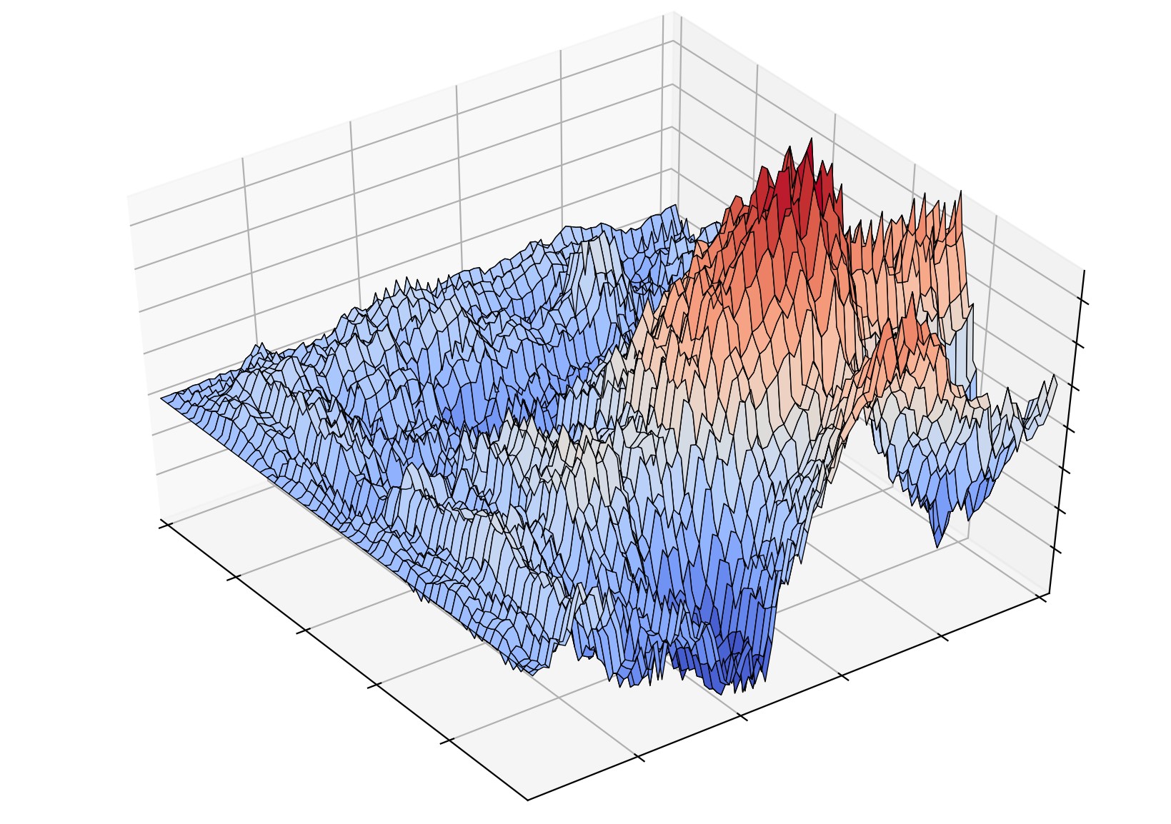
As an example application of theorem 2, we can construct generalisations of Brownian motion varying over a multidimensional index set. The 2-dimensional case is called a Brownian sheet, and a sample is plotted in figure 2 above. This can represent a continuous random path, which itself varies randomly over time. Such processes may be used to build models of interest rates where, at any moment in time, we have an entire yield curve representing the interest rates for all maturities, and these also vary randomly over time.
Lemma 3 For each positive integer d, there exists a zero mean Gaussian stochastic process
with covariance
for all
. This has a continuous modification, which is locally
![\displaystyle {\mathbb E}[W_sW_t]=\prod_{i=1}^d s_i\wedge t_i,](https://s0.wp.com/latex.php?latex=%5Cdisplaystyle++%7B%5Cmathbb+E%7D%5BW_sW_t%5D%3D%5Cprod_%7Bi%3D1%7D%5Ed+s_i%5Cwedge+t_i%2C+&bg=ffffff&fg=000000&s=0&c=20201002)
Proof: I make use of the standard result that, for any (real) inner product space V, we can define a joint normal collection of random variables 

![{{\mathbb E}[X(u)X(v)]=\langle u,v\rangle}](https://s0.wp.com/latex.php?latex=%7B%7B%5Cmathbb+E%7D%5BX%28u%29X%28v%29%5D%3D%5Clangle+u%2Cv%5Crangle%7D&bg=ffffff&fg=000000&s=0&c=20201002)

![\displaystyle \sum_{i,j=1}^nc_ic_j{\mathbb E}[X(v_i)X(v_j)]=\left\langle\sum_{i=1}^nc_iv_i,\sum_{j=1}^nc_jv_j\right\rangle\ge0.](https://s0.wp.com/latex.php?latex=%5Cdisplaystyle++%5Csum_%7Bi%2Cj%3D1%7D%5Enc_ic_j%7B%5Cmathbb+E%7D%5BX%28v_i%29X%28v_j%29%5D%3D%5Cleft%5Clangle%5Csum_%7Bi%3D1%7D%5Enc_iv_i%2C%5Csum_%7Bj%3D1%7D%5Enc_jv_j%5Cright%5Crangle%5Cge0.+&bg=ffffff&fg=000000&s=0&c=20201002) |
Take V to be 

 |
for all 


![\displaystyle \begin{aligned} {\mathbb E}[W_sW_t]&=\int 1_{[0,s)}1_{[0,t)}d\lambda\\ &=\int\cdots\int 1_{\{u_1 < s_1\wedge t_1,\ldots,u_d < s_d\wedge t_d\}}du_1\cdots du_d\\ &=\prod_{i=1}^d s_i\wedge t_i \end{aligned}](https://s0.wp.com/latex.php?latex=%5Cdisplaystyle++%5Cbegin%7Baligned%7D+%7B%5Cmathbb+E%7D%5BW_sW_t%5D%26%3D%5Cint+1_%7B%5B0%2Cs%29%7D1_%7B%5B0%2Ct%29%7Dd%5Clambda%5C%5C+%26%3D%5Cint%5Ccdots%5Cint+1_%7B%5C%7Bu_1+%3C+s_1%5Cwedge+t_1%2C%5Cldots%2Cu_d+%3C+s_d%5Cwedge+t_d%5C%7D%7Ddu_1%5Ccdots+du_d%5C%5C+%26%3D%5Cprod_%7Bi%3D1%7D%5Ed+s_i%5Cwedge+t_i+%5Cend%7Baligned%7D+&bg=ffffff&fg=000000&s=0&c=20201002) |
as required.
It remains to show that W has a modification with the stated Hölder continuity and, for this, it is sufficient to prove the result for index t restricted to bounded sets of the form ![{[0,T]^d}](https://s0.wp.com/latex.php?latex=%7B%5B0%2CT%5D%5Ed%7D&bg=ffffff&fg=000000&s=0&c=20201002)
![{s,t\in[0,T]^d}](https://s0.wp.com/latex.php?latex=%7Bs%2Ct%5Cin%5B0%2CT%5D%5Ed%7D&bg=ffffff&fg=000000&s=0&c=20201002)
![\displaystyle \begin{aligned} {\mathbb E}[(W_s-W_t)^2]&= \int\left(1_{[0,s)}-1_{[0,t)}\right)^2d\lambda\\ &\le\sum_{i=1}^d\int \prod_{j\not=i}1_{\{u_j < T\}}1_{\{s_i\wedge t_i\le u_i\le s_i\vee t_i\}}d\lambda(u)\\ &=T^{d-1}\sum_{i=1}^d\lvert t_i-s_i\rvert\\ &=T^{d-1}\lVert t-s\rVert_1. \end{aligned}](https://s0.wp.com/latex.php?latex=%5Cdisplaystyle++%5Cbegin%7Baligned%7D+%7B%5Cmathbb+E%7D%5B%28W_s-W_t%29%5E2%5D%26%3D+%5Cint%5Cleft%281_%7B%5B0%2Cs%29%7D-1_%7B%5B0%2Ct%29%7D%5Cright%29%5E2d%5Clambda%5C%5C+%26%5Cle%5Csum_%7Bi%3D1%7D%5Ed%5Cint+%5Cprod_%7Bj%5Cnot%3Di%7D1_%7B%5C%7Bu_j+%3C+T%5C%7D%7D1_%7B%5C%7Bs_i%5Cwedge+t_i%5Cle+u_i%5Cle+s_i%5Cvee+t_i%5C%7D%7Dd%5Clambda%28u%29%5C%5C+%26%3DT%5E%7Bd-1%7D%5Csum_%7Bi%3D1%7D%5Ed%5Clvert+t_i-s_i%5Crvert%5C%5C+%26%3DT%5E%7Bd-1%7D%5ClVert+t-s%5CrVert_1.+%5Cend%7Baligned%7D+&bg=ffffff&fg=000000&s=0&c=20201002) |
Hence, for any fixed 
![\displaystyle {\mathbb E}[\lvert W_s-W_t\rvert^\alpha]\le C\lVert t-s\rVert_1^{\alpha/2}.](https://s0.wp.com/latex.php?latex=%5Cdisplaystyle++%7B%5Cmathbb+E%7D%5B%5Clvert+W_s-W_t%5Crvert%5E%5Calpha%5D%5Cle+C%5ClVert+t-s%5CrVert_1%5E%7B%5Calpha%2F2%7D.+&bg=ffffff&fg=000000&s=0&c=20201002) |
Theorem 2 can be applied so long as 


Proof of the Continuity Theorem
To show that a process
 |
In particular, this should be bounded of the form 

![\displaystyle \begin{aligned} {\mathbb E}\left[\sup_{\lVert x-y\rVert < \epsilon}d(U_x,U_y)^\alpha\right] &\le\sum_{\lVert x-y\rVert < \epsilon}{\mathbb E}\left[d(U_x,U_y)^\alpha\right]\\ &\le\sum_{\lVert x-y\rVert < \epsilon}C\epsilon^{d+\beta}. \end{aligned}](https://s0.wp.com/latex.php?latex=%5Cdisplaystyle++%5Cbegin%7Baligned%7D+%7B%5Cmathbb+E%7D%5Cleft%5B%5Csup_%7B%5ClVert+x-y%5CrVert+%3C+%5Cepsilon%7Dd%28U_x%2CU_y%29%5E%5Calpha%5Cright%5D+%26%5Cle%5Csum_%7B%5ClVert+x-y%5CrVert+%3C+%5Cepsilon%7D%7B%5Cmathbb+E%7D%5Cleft%5Bd%28U_x%2CU_y%29%5E%5Calpha%5Cright%5D%5C%5C+%26%5Cle%5Csum_%7B%5ClVert+x-y%5CrVert+%3C+%5Cepsilon%7DC%5Cepsilon%5E%7Bd%2B%5Cbeta%7D.+%5Cend%7Baligned%7D+&bg=ffffff&fg=000000&s=0&c=20201002) |
In cases of interest, the set S will be infinite, and the sum on the right hand side will contain infinitely many terms, so will diverge. As it is, this is not much help. However, if we restrict x and y to lie on a regular grid whose spacing is of order 


Lemma 4 Let E be a separable complete metric space, S be a subset of the unit d-cube
, and
Then, there exists a countable dense subset
such that, with probability one,
is
for all
. In particular, the
satisfies
.
Proof: For each nonnegative integer n, we let 


Moving from 1 dimension to d dimensions, we let 
 |
We note that, for each n, these sets form a partition of 


 |
Note that, whatever the choice of 


Consider the random variables,
 |
We note that there are at most 


![\displaystyle \begin{aligned} {\mathbb E}\left[Y_n^\alpha\right] &\le\sum_{ x\in\mathbb{\tilde D}_n^d,\ y\in\mathbb{\tilde D}_{n+1}^d\cap I_n(x) }{\mathbb E}\left[d(U_{\theta_n(x)},U_{\theta_{n+1}(y)})^\alpha\right]\\ &\le C2^{nd}2^d2^{-n(d+\beta)}=C2^d2^{-n\beta},\\ {\mathbb E}\left[Z_n^\alpha\right] &\le\sum_{x,y\in\mathbb{\tilde D}_n^k,\ \lVert x-y\rVert_\infty\le2^{-n}}{\mathbb E}\left[d(U_{\theta_n(x)},U_{\theta_n(y)})^\alpha\right]\\ &\le C2^{nd}3^d2^{(1-n)(d+\beta)} =C6^d2^{-(n-1)\beta}. \end{aligned}](https://s0.wp.com/latex.php?latex=%5Cdisplaystyle++%5Cbegin%7Baligned%7D+%7B%5Cmathbb+E%7D%5Cleft%5BY_n%5E%5Calpha%5Cright%5D+%26%5Cle%5Csum_%7B+x%5Cin%5Cmathbb%7B%5Ctilde+D%7D_n%5Ed%2C%5C+y%5Cin%5Cmathbb%7B%5Ctilde+D%7D_%7Bn%2B1%7D%5Ed%5Ccap+I_n%28x%29+%7D%7B%5Cmathbb+E%7D%5Cleft%5Bd%28U_%7B%5Ctheta_n%28x%29%7D%2CU_%7B%5Ctheta_%7Bn%2B1%7D%28y%29%7D%29%5E%5Calpha%5Cright%5D%5C%5C+%26%5Cle+C2%5E%7Bnd%7D2%5Ed2%5E%7B-n%28d%2B%5Cbeta%29%7D%3DC2%5Ed2%5E%7B-n%5Cbeta%7D%2C%5C%5C+%7B%5Cmathbb+E%7D%5Cleft%5BZ_n%5E%5Calpha%5Cright%5D+%26%5Cle%5Csum_%7Bx%2Cy%5Cin%5Cmathbb%7B%5Ctilde+D%7D_n%5Ek%2C%5C+%5ClVert+x-y%5CrVert_%5Cinfty%5Cle2%5E%7B-n%7D%7D%7B%5Cmathbb+E%7D%5Cleft%5Bd%28U_%7B%5Ctheta_n%28x%29%7D%2CU_%7B%5Ctheta_n%28y%29%7D%29%5E%5Calpha%5Cright%5D%5C%5C+%26%5Cle+C2%5E%7Bnd%7D3%5Ed2%5E%7B%281-n%29%28d%2B%5Cbeta%29%7D+%3DC6%5Ed2%5E%7B-%28n-1%29%5Cbeta%7D.+%5Cend%7Baligned%7D+&bg=ffffff&fg=000000&s=0&c=20201002) |
Consequently, for 

![\displaystyle \begin{aligned} &{\mathbb E}\left[\tilde Y_n^\alpha\right]\le C2^d2^{-n(\beta-\alpha\gamma)},\\ &{\mathbb E}\left[\tilde Z_n^\alpha\right]\le C6^d2^{\beta-n(\beta-\alpha\gamma)}. \end{aligned}](https://s0.wp.com/latex.php?latex=%5Cdisplaystyle++%5Cbegin%7Baligned%7D+%26%7B%5Cmathbb+E%7D%5Cleft%5B%5Ctilde+Y_n%5E%5Calpha%5Cright%5D%5Cle+C2%5Ed2%5E%7B-n%28%5Cbeta-%5Calpha%5Cgamma%29%7D%2C%5C%5C+%26%7B%5Cmathbb+E%7D%5Cleft%5B%5Ctilde+Z_n%5E%5Calpha%5Cright%5D%5Cle+C6%5Ed2%5E%7B%5Cbeta-n%28%5Cbeta-%5Calpha%5Cgamma%29%7D.+%5Cend%7Baligned%7D+&bg=ffffff&fg=000000&s=0&c=20201002) |
By the sums of geometric series, these have bounded sum over n. For distinct 

 |
Also, choose 


 |
Hence, the
 |
Raising to the power of
 |
which has finite expectation, as required. ⬜
This is the hard part of the proof over with now. Constructing the continuous modification over bounded index sets is straightforward.
Lemma 5 Let E be a separable and complete metric space,
Proof: By scaling, if necessary, we can suppose without loss of generality that S is contained in the unit d-cube 


 |
By uniform continuity, the limit over y exists and defines a 

![\displaystyle \begin{aligned} {\mathbb E}[d(U_x,\tilde U_x)^\alpha] &\le\liminf_{n\rightarrow\infty}{\mathbb E}[d(U_x,U_{x_n})^\alpha]\\ &\le\lim_{n\rightarrow\infty}C\lVert x-x_n\rVert^{d+\beta}\\ &=0. \end{aligned}](https://s0.wp.com/latex.php?latex=%5Cdisplaystyle++%5Cbegin%7Baligned%7D+%7B%5Cmathbb+E%7D%5Bd%28U_x%2C%5Ctilde+U_x%29%5E%5Calpha%5D+%26%5Cle%5Climinf_%7Bn%5Crightarrow%5Cinfty%7D%7B%5Cmathbb+E%7D%5Bd%28U_x%2CU_%7Bx_n%7D%29%5E%5Calpha%5D%5C%5C+%26%5Cle%5Clim_%7Bn%5Crightarrow%5Cinfty%7DC%5ClVert+x-x_n%5CrVert%5E%7Bd%2B%5Cbeta%7D%5C%5C+%26%3D0.+%5Cend%7Baligned%7D+&bg=ffffff&fg=000000&s=0&c=20201002) |
Hence 

Completing the proof by extending to unbounded index sets is now almost a formality.
Proof of Theorem 2: For each positive integer n, let 


 |
This is clearly 

when we apply Kolmogorov continuity thm, do we require process X_t to be separable?
I’m not sure what you mean by X_t is separable. We do require the metric space in which X takes values to be separable. This is only so that d(X_s,X_t) is a measurable random variable. Even if the metric space is not separable, but you know that these random variables are measurable, then the theorem still works. Even if it is not measurable, so that the probabilities are not even defined, the theorem will still work as long as you interpret the probabilities as outer measures.
Great! Thank you for the explanation!
Thanks a lot for your post. One can easily show that Theorem 1 is sharp. For example, define a real-valued stochastic process as X(t) = I_{U =< t } for all t \in [0,1], where "I" is the indicator function and U is a uniformly distributed random variable on the range [0,1]. Then we have E [ |X(t)-X(s)|^\alpha ] = |t-s| for all \alpha but obviously X has no continuous sample paths. Do you know an example that shows Theorem 2 is also sharp for example for the case d = 2? Thank you in advance!