Optional Sampling

Doob’s optional sampling theorem states that the properties of martingales, submartingales and supermartingales generalize to stopping times. For simple stopping times, which take only finitely many values in ${{\mathbb R}_+}$ , the argument is a relatively basic application of elementary integrals. For simple stopping times ${\sigma\le\tau}$ , the stochastic interval ${(\sigma,\tau]}$ and its indicator function ${1_{(\sigma,\tau]}}$ are elementary predictable. For any submartingale ${X}$ , the properties of elementary integrals give the inequality

$\displaystyle {\mathbb E}\left[X_\tau-X_\sigma\right]={\mathbb E}\left[\int_0^\infty 1_{(\sigma,\tau]}\,dX\right]\ge 0.$

(1)

For a set ${A\in \mathcal{F}_\sigma}$ the following

$\displaystyle \sigma^\prime(\omega)=\begin{cases} \sigma(\omega),&\textrm{if }\omega\in A,\\ \tau(\omega),&\textrm{otherwise}, \end{cases}$

is easily seen to be a stopping time. Replacing ${\sigma}$ by ${\sigma^\prime}$ extends inequality (1) to the following,

$\displaystyle {\mathbb E}\left[1_A(X_\tau-X_\sigma)\right]={\mathbb E}\left[X_\tau-X_{\sigma^\prime}\right]\ge 0.$

(2)

As this inequality holds for all sets ${A\in\mathcal{F}_\sigma}$ it implies the extension of the submartingale property ${X_\sigma\le{\mathbb E}[X_\tau\vert\mathcal{F}_\sigma]}$ to the random times. This argument applies to all simple stopping times, and is sufficient to prove the optional sampling result for discrete time submartingales. In continuous time, the additional hypothesis that the process is right-continuous is required. Then, the result follows by taking limits of simple stopping times.

Theorem 1 Let ${\sigma\le\tau}$ be bounded stopping times. For any cadlag martingale, submartingale or supermartingale ${X}$ , the random variables ${X_\sigma, X_\tau}$ are integrable and the following are satisfied.

If ${X}$ is a martingale then, ${X_\sigma={\mathbb E}\left[X_{\tau}\vert\mathcal{F}_\sigma\right].}$

If ${X}$ is a submartingale then, ${X_\sigma\le{\mathbb E}\left[X_{\tau}\vert\mathcal{F}_\sigma\right].}$

If ${X}$ is a supermartingale then, ${X_\sigma\ge{\mathbb E}\left[X_{\tau}\vert\mathcal{F}_\sigma\right].}$

Continue reading “Optional Sampling” →

Cadlag Modifications

As was mentioned in the initial post of these stochastic calculus notes, it is important to choose good versions of stochastic processes. In some cases, such as with Brownian motion, it is possible to explicitly construct the process to be continuous. However, in many more cases, it is necessary to appeal to more general results to assure the existence of such modifications.

The theorem below guarantees that many of the processes studied in stochastic calculus have a right-continuous version and, furthermore, these versions necessarily have left limits everywhere. Such processes are known as càdlàg from the French for “continu à droite, limites à gauche” (I often drop the accents, as seems common). Alternative terms used to refer to a cadlag process are rcll (right-continuous with left limits), R-process and right process. For a cadlag process ${X}$ , the left limit at any time ${t>0}$ is denoted by ${X_{t-}}$ (and ${X_{0-}\equiv X_0}$ ). The jump at time ${t}$ is denoted by ${\Delta X_t=X_t-X_{t-}}$ .

We work with respect to a complete filtered probability space ${(\Omega,\mathcal{F},\{\mathcal{F}_t\}_{t\ge 0},{\mathbb P})}$ .

Theorem 1 below provides us with cadlag versions under the condition that elementary integrals of the processes cannot, in a sense, get too large. Recall that elementary predictable processes are of the form

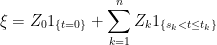
$\displaystyle \xi=Z_01_{\{t=0\}}+\sum_{k=1}^nZ_k1_{\{s_k<t\le t_k\}}$

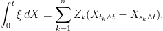
for times ${s_k<t_k}$ , ${\mathcal{F}_0}$ -measurable random variable ${Z_0}$ and ${\mathcal{F}_{s_k}}$ -measurable random variables ${Z_k}$ . Its integral with respect to a stochastic process ${X}$ is

$\displaystyle \int_0^t \xi\,dX=\sum_{k=1}^nZ_k(X_{t_k\wedge t}-X_{s_{k}\wedge t}).$

An elementary predictable set is a subset of ${{\mathbb R}_+\times\Omega}$ which is a finite union of sets of the form ${\{0\}\times F}$ for ${F\in\mathcal{F}_0}$ and ${(s,t]\times F}$ for nonnegative reals ${s<t}$ and ${F\in\mathcal{F}_s}$ . Then, a process is an indicator function ${1_A}$ of some elementary predictable set ${A}$ if and only if it is elementary predictable and takes values in ${\{0,1\}}$ .

The following theorem guarantees the existence of cadlag versions for many types of processes. The first statement applies in particular to martingales, submartingales and supermartingales, whereas the second statement is important for the study of general semimartingales.

Theorem 1 Let X be an adapted stochastic process which is right-continuous in probability and such that either of the following conditions holds. Then, it has a cadlag version.

X is integrable and, for every ${t\in{\mathbb R}_+}$ ,
$\displaystyle \left\{{\mathbb E}\left[\int_0^t1_A\,dX\right]\colon A\textrm{ is elementary}\right\}$

is bounded.

For every ${t\in{\mathbb R}_+}$ the set
$\displaystyle \left\{\int_0^t1_A\,dX\colon A\textrm{ is elementary}\right\}$

is bounded in probability.

Continue reading “Cadlag Modifications” →

Upcrossings, Downcrossings, and Martingale Convergence

The number of times that a process passes upwards or downwards through an interval is refered to as the number of upcrossings and respectively the number of downcrossings of the process.

Consider a process ${X_t}$ whose time index ${t}$ runs through an index set ${\mathbb{T}\subseteq{\mathbb R}}$ . For real numbers ${a<b}$ , the number of upcrossings of ${X}$ across the interval ${[a,b]}$ is the supremum of the nonnegative integers ${n}$ such that there exists times ${s_k,t_k\in\mathbb{T}}$ satisfying

$\displaystyle s_1<t_1<s_2<t_2<\cdots<s_n<t_n$

(1)

and for which ${X_{s_k}\le a<b\le X_{t_k}}$ . The number of upcrossings is denoted by ${U[a,b]}$ , which is either a nonnegative integer or is infinite. Similarly, the number of downcrossings, denoted by ${D[a,b]}$ , is the supremum of the nonnegative integers ${n}$ such that there are times ${s_k,t_k\in\mathbb{T}}$ satisfying (1) and such that ${X_{s_k}\ge b>a\ge X_{t_k}}$ .

Note that between any two upcrossings there is a downcrossing and, similarly, between any two downcrossings there is an upcrossing. It follows that ${U[a,b]}$ and ${D[a,b]}$ can differ by at most 1, and they are either both finite or both infinite.

The significance of the upcrossings of a process to convergence results is due to the following criterion for convergence of a sequence.

Theorem 1 A sequence ${x_1,x_2,\ldots}$ converges to a limit in the extended real numbers if and only if the number of upcrossings ${U[a,b]}$ is finite for all ${a<b}$ .

Continue reading “Upcrossings, Downcrossings, and Martingale Convergence” →

Martingales and Elementary Integrals

A martingale is a stochastic process which stays the same, on average. That is, the expected future value conditional on the present is equal to the current value. Examples include the wealth of a gambler as a function of time, assuming that he is playing a fair game. The canonical example of a continuous time martingale is Brownian motion and, in discrete time, a symmetric random walk is a martingale. As always, we work with respect to a filtered probability space ${(\Omega,\mathcal{F},\{\mathcal{F}_t\}_{t\ge 0},{\mathbb P})}$ . A process ${X}$ is said to be integrable if the random variables ${X_t}$ are integrable, so that ${{\mathbb E}[\vert X_t\vert]<\infty}$ .

Definition 1 A martingale, ${X}$ , is an integrable process satisfying

$\displaystyle X_s={\mathbb E}[X_t\mid\mathcal{F}_s]$

for all ${s<t\in{\mathbb R}_+}$ .

Continue reading “Martingales and Elementary Integrals” →

	Anonymous on About
	Anonymous on About
	Anonymous on The Stochastic Integral
	Anonymous on Bessel Processes
	Anonymous on Bessel Processes
	Stat Prof on Pathwise Regularity of Optiona…
	Yang Chu on Spitzer’s Formula
	Anonymous on About
	Anonymous on Continuous Processes with Inde…
	Anonymous on Continuous Processes with Inde…