Rao’s Quasimartingale Decomposition

In this post I’ll give a proof of Rao’s decomposition for quasimartingales. That is, every quasimartingale decomposes as the sum of a submartingale and a supermartingale. Equivalently, every quasimartingale is a difference of two submartingales, or alternatively, of two supermartingales. This was originally proven by Rao (Quasi-martingales, 1969), and is an important result in the general theory of continuous-time stochastic processes.

As always, we work with respect to a filtered probability space ${(\Omega,\mathcal{F},\{\mathcal{F}_t\}_{t\ge0},{\mathbb P})}$ . It is not required that the filtration satisfies either of the usual conditions — the filtration need not be complete or right-continuous. The methods used in this post are elementary, requiring only basic measure theory along with the definitions and first properties of martingales, submartingales and supermartingales. Other than referring to the definitions of quasimartingales and mean variation given in the previous post, there is no dependency on any of the general theory of semimartingales, nor on stochastic integration other than for elementary integrands.

Recall that, for an adapted integrable process X, the mean variation on an interval ${[0,t]}$ is

$\displaystyle {\rm Var}_t(X)=\sup{\mathbb E}\left[\int_0^t\xi\,dX\right],$

where the supremum is taken over all elementary processes ${\xi}$ with ${\vert\xi\vert\le1}$ . Then, X is a quasimartingale if and only if ${{\rm Var}_t(X)}$ is finite for all positive reals t. It was shown that all supermartingales are quasimartingales with mean variation given by

$\displaystyle {\rm Var}_t(X)={\mathbb E}\left[X_0-X_t\right].$

(1)

Rao’s decomposition can be stated in several different ways, depending on what conditions are required to be satisfied by the quasimartingale X. As the definition of quasimartingales does differ between texts, there are different versions of Rao’s theorem around although, up to martingale terms, they are equivalent. In this post, I’ll give three different statements with increasingly stronger conditions for X. First, the following statement applies to all quasimartingales as defined in these notes. Theorem 1 can be compared to the Jordan decomposition, which says that any function ${f\colon{\mathbb R}_+\rightarrow{\mathbb R}}$ with finite variation on bounded intervals can be decomposed as the difference of increasing functions or, equivalently, of decreasing functions. Replacing finite variation functions by quasimartingales and decreasing functions by supermartingales gives the following.

Theorem 1 (Rao) A process X is a quasimartingale if and only if it decomposes as

$\displaystyle X=Y-Z$ (2)

for supermartingales Y and Z. Furthermore,

this decomposition can be done in a minimal sense, so that if ${X=Y^\prime-Z^\prime}$ is any other such decomposition then ${Y^\prime-Y=Z^\prime-Z}$ is a supermartingale.

the inequality

$\displaystyle {\rm Var}_t(X)\le{\mathbb E}[Y_0-Y_t]+{\mathbb E}[Z_0-Z_t],$ (3)

holds, with equality for all ${t\ge0}$ if and only if the decomposition is minimal.

the minimal decomposition is unique up to a martingale. That is, if ${X=Y-Z=Y^\prime-Z^\prime}$ are two such minimal decompositions, then ${Y^\prime-Y=Z^\prime-Z}$ is a martingale.

Continue reading “Rao’s Quasimartingale Decomposition” →

Quasimartingales

Quasimartingales are a natural generalization of martingales, submartingales and supermartingales. They were first introduced by Fisk in order to extend the Doob-Meyer decomposition to a larger class of processes, showing that continuous quasimartingales can be decomposed into martingale and finite variation terms (Quasi-martingales, 1965). This was later extended to right-continuous processes by Orey (F-Processes, 1967). The way in which quasimartingales relate to sub- and super-martingales is very similar to how functions of finite variation relate to increasing and decreasing functions. In particular, by the Jordan decomposition, any finite variation function on an interval decomposes as the sum of an increasing and a decreasing function. Similarly, a stochastic process is a quasimartingale if and only if it can be written as the sum of a submartingale and a supermartingale. This important result was first shown by Rao (Quasi-martingales, 1969), and means that much of the theory of submartingales can be extended without much work to also cover quasimartingales.

Often, given a process, it is important to show that it is a semimartingale so that the techniques of stochastic calculus can be applied. If there is no obvious decomposition into local martingale and finite variation terms, then, one way of doing this is to show that it is a quasimartingale. All right-continuous quasimartingales are semimartingales. This result is also important in the general theory of semimartingales with, for example, many proofs of the Bichteler-Dellacherie theorem involving quasimartingales.

In this post, I will mainly be concerned with the definition and very basic properties of quasimartingales, and look at the more advanced theory in the following post. We work with respect to a filtered probability space ${(\Omega,\mathcal{F},\{\mathcal{F}_t\}_{t\ge0},{\mathbb P})}$ . It is not necessary to assume that either of the usual conditions, of right-continuity or completeness, hold. First, the mean variation of a process is defined as follows.

Definition 1 The mean variation of an integrable stochastic process X on an interval ${[0,t]}$ is

$\displaystyle {\rm Var}_t(X)=\sup{\mathbb E}\left[\sum_{k=1}^n\left\vert{\mathbb E}\left[X_{t_k}-X_{t_{k-1}}\;\vert\mathcal{F}_{t_{k-1}}\right]\right\vert\right].$ (1)

Here, the supremum is taken over all finite sequences of times,

$\displaystyle 0=t_0\le t_1\le\cdots\le t_n=t.$

A quasimartingale, then, is a process with finite mean variation on each bounded interval.

Definition 2 A quasimartingale, X, is an integrable adapted process such that ${{\rm Var}_t(X)}$ is finite for each time ${t\in{\mathbb R}_+}$ .

Continue reading “Quasimartingales” →

Failure of the Martingale Property

In this post, I give an example of a class of processes which can be expressed as integrals with respect to Brownian motion, but are not themselves martingales. As stochastic integration preserves the local martingale property, such processes are guaranteed to be at least local martingales. However, this is not enough to conclude that they are proper martingales. Whereas constructing examples of local martingales which are not martingales is a relatively straightforward exercise, such examples are often slightly contrived and the martingale property fails for obvious reasons (e.g., double-loss betting strategies). The aim here is to show that the martingale property can fail for very simple stochastic differential equations which are likely to be met in practice, and it is not always obvious when this situation arises.

Consider the following stochastic differential equation

$\displaystyle \setlength\arraycolsep{2pt} \begin{array}{rl} &\displaystyle dX = aX^c\,dB +b X dt,\smallskip\\ &\displaystyle X_0=x, \end{array}$

(1)

for a nonnegative process X. Here, B is a Brownian motion and a,b,c,x are positive constants. This a common SDE appearing, for example, in the constant elasticity of variance model for option pricing. Now consider the following question: what is the expected value of X at time t?

The obvious answer seems to be that ${{\mathbb E}[X_t]=xe^{bt}}$ , based on the idea that X has growth rate b on average. A more detailed argument is to write out (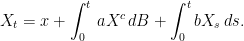1) in integral form

$\displaystyle X_t=x+\int_0^t\,aX^c\,dB+ \int_0^t bX_s\,ds.$

(2)

The next step is to note that the first integral is with respect to Brownian motion, so has zero expectation. Therefore,

$\displaystyle {\mathbb E}[X_t]=x+\int_0^tb{\mathbb E}[X_s]\,ds.$

This can be differentiated to obtain the ordinary differential equation ${d{\mathbb E}[X_t]/dt=b{\mathbb E}[X_t]}$ , which has the unique solution ${{\mathbb E}[X_t]={\mathbb E}[X_0]e^{bt}}$ .

In fact this argument is false. For ${c\le1}$ there is no problem, and ${{\mathbb E}[X_t]=xe^{bt}}$ as expected. However, for all ${c>1}$ the conclusion is wrong, and the strict inequality ${{\mathbb E}[X_t]<xe^{bt}}$ holds.

The point where the argument above falls apart is the statement that the first integral in (2) has zero expectation. This would indeed follow if it was known that it is a martingale, as is often assumed to be true for stochastic integrals with respect to Brownian motion. However, stochastic integration preserves the local martingale property and not, in general, the martingale property itself. If ${c>1}$ then we have exactly this situation, where only the local martingale property holds. The first integral in (2) is not a proper martingale, and has strictly negative expectation at all positive times. The reason that the martingale property fails here for ${c>1}$ is that the coefficient ${aX^c}$ of dB grows too fast in X.

In this post, I will mainly be concerned with the special case of (1) with a=1 and zero drift.

$\displaystyle \setlength\arraycolsep{2pt} \begin{array}{rl} &\displaystyle dX=X^c\,dB,\smallskip\\ &\displaystyle X_0=x. \end{array}$

(3)

The general form (1) can be reduced to this special case, as I describe below. SDEs (1) and (3) do have unique solutions, as I will prove later. Then, as X is a nonnegative local martingale, if it ever hits zero then it must remain there (0 is an absorbing boundary).

The solution X to (3) has the following properties, which will be proven later in this post.

If ${c\le1}$ then X is a martingale and, for ${c<1}$ , it eventually hits zero with probability one.
If ${c>1}$ then X is a strictly positive local martingale but not a martingale. In fact, the following inequality holds

$\displaystyle {\mathbb E}[X_t\mid\mathcal{F}_s]<X_s$ (4)

(almost surely) for times ${s<t}$ . Furthermore, for any positive constant ${p<2c-1}$ , ${{\mathbb E}[X_t^p]}$ is bounded over ${t\ge0}$ and tends to zero as ${t\rightarrow\infty}$ .

Continue reading “Failure of the Martingale Property” →

Local Martingales

Recall from the previous post that a cadlag adapted process ${X}$ is a local martingale if there is a sequence ${\tau_n}$ of stopping times increasing to infinity such that the stopped processes ${1_{\{\tau_n>0\}}X^{\tau_n}}$ are martingales. Local submartingales and local supermartingales are defined similarly.

An example of a local martingale which is not a martingale is given by the `double-loss’ gambling strategy. Interestingly, in 18th century France, such strategies were known as martingales and is the origin of the mathematical term. Suppose that a gambler is betting sums of money, with even odds, on a simple win/lose game. For example, betting that a coin toss comes up heads. He could bet one dollar on the first toss and, if he loses, double his stake to two dollars for the second toss. If he loses again, then he is down three dollars and doubles the stake again to four dollars. If he keeps on doubling the stake after each loss in this way, then he is always gambling one more dollar than the total losses so far. He only needs to continue in this way until the coin eventually does come up heads, and he walks away with net winnings of one dollar. This therefore describes a fair game where, eventually, the gambler is guaranteed to win.

Of course, this is not an effective strategy in practise. The losses grow exponentially and, if he doesn’t win quickly, the gambler must hit his credit limit in which case he loses everything. All that the strategy achieves is to trade a large probability of winning a dollar against a small chance of losing everything. It does, however, give a simple example of a local martingale which is not a martingale.

The gamblers winnings can be defined by a stochastic process ${\{Z_n\}_{n=1,\ldots}}$ representing his net gain (or loss) just before the n’th toss. Let ${\epsilon_1,\epsilon_2,\ldots}$ be a sequence of independent random variables with ${{\mathbb P}(\epsilon_n=1)={\mathbb P}(\epsilon_n=-1)=1/2}$ . Here, ${\epsilon_n}$ represents the outcome of the n’th toss, with 1 referring to a head and -1 referring to a tail. Set ${Z_1=0}$ and

$\displaystyle Z_{n}=\begin{cases} 1,&\text{if }Z_{n-1}=1,\\ Z_{n-1}+\epsilon_n(1-Z_{n-1}),&\text{otherwise}. \end{cases}$

This is a martingale with respect to its natural filtration, starting at zero and, eventually, ending up equal to one. It can be converted into a local martingale by speeding up the time scale to fit infinitely many tosses into a unit time interval

$\displaystyle X_t=\begin{cases} Z_n,&\text{if }1-1/n\le t<1-1/(n+1),\\ 1,&\text{if }t\ge 1. \end{cases}$

This is a martingale with respect to its natural filtration on the time interval ${[0,1)}$ . Letting ${\tau_n=\inf\{t\colon\vert X_t\vert\ge n\}}$ then the optional stopping theorem shows that ${X^{\tau_n}_t}$ is a uniformly bounded martingale on ${t<1}$ , continuous at ${t=1}$ , and constant on ${t\ge 1}$ . This is therefore a martingale, showing that ${X}$ is a local martingale. However, ${{\mathbb E}[X_1]=1\not={\mathbb E}[X_0]=0}$ , so it is not a martingale. Continue reading “Local Martingales” →

Localization

Special classes of processes, such as martingales, are very important to the study of stochastic calculus. In many cases, however, processes under consideration `almost’ satisfy the martingale property, but are not actually martingales. This occurs, for example, when taking limits or stochastic integrals with respect to martingales. It is necessary to generalize the martingale concept to that of local martingales. More generally, localization is a method of extending a given property to a larger class of processes. In this post I mention a few definitions and simple results concerning localization, and look more closely at local martingales in the next post.

Definition 1 Let P be a class of stochastic processes. Then, a process X is locally in P if there exists a sequence of stopping times ${\tau_n\uparrow\infty}$ such that the stopped processes

$\displaystyle 1_{\{\tau_n>0\}}X^{\tau_n}$

are in P. The sequence ${\tau_n}$ is called a localizing sequence for X (w.r.t. P).

I write ${P_{\rm loc}}$ for the processes locally in P. Choosing the sequence ${\tau_n\equiv\infty}$ of stopping times shows that ${P\subseteq P_{\rm loc}}$ . A class of processes is said to be stable if ${1_{\{\tau>0\}}X^\tau}$ is in P whenever X is, for all stopping times ${\tau}$ . For example, the optional stopping theorem shows that the classes of cadlag martingales, cadlag submartingales and cadlag supermartingales are all stable.

Definition 2 A process is a

a local martingale if it is locally in the class of cadlag martingales.

a local submartingale if it is locally in the class of cadlag submartingales.

a local supermartingale if it is locally in the class of cadlag supermartingales.

Continue reading “Localization” →

Martingale Convergence

The martingale property is strong enough to ensure that, under relatively weak conditions, we are guaranteed convergence of the processes as time goes to infinity. In a previous post, I used Doob’s upcrossing inequality to show that, with probability one, discrete-time martingales will converge at infinity under the extra condition of ${L^1}$ -boundedness. Here, I consider continuous-time martingales. This is a more general situation, because it considers limits as time runs through the uncountably infinite set of positive reals instead of the countable set of positive integer times. Although these results can also be proven in a similar way by counting the upcrossings of a process, I instead show how they follow directly from the existence of cadlag modifications. We work with respect to a complete filtered probability space ${(\Omega,\mathcal{F},\{\mathcal{F}_t\}_{t\ge 0},{\mathbb P})}$ .

Recall that a stochastic process ${X}$ is ${L^1}$ -bounded if the set ${\{X_t\colon t\in{\mathbb R}_+\}}$ is ${L^1}$ -bounded. That is, ${{\mathbb E}|X_t|}$ is bounded above by some finite value as ${t}$ runs through the positive reals.

Theorem 1 Let ${X}$ be a cadlag and ${L^1}$ -bounded martingale (or submartingale, or supermartingale). Then, the limit ${X_\infty=\lim_{t\rightarrow\infty}X_t}$ exists and is finite, with probability one.

Continue reading “Martingale Convergence” →

Optional Sampling

Doob’s optional sampling theorem states that the properties of martingales, submartingales and supermartingales generalize to stopping times. For simple stopping times, which take only finitely many values in ${{\mathbb R}_+}$ , the argument is a relatively basic application of elementary integrals. For simple stopping times ${\sigma\le\tau}$ , the stochastic interval ${(\sigma,\tau]}$ and its indicator function ${1_{(\sigma,\tau]}}$ are elementary predictable. For any submartingale ${X}$ , the properties of elementary integrals give the inequality

$\displaystyle {\mathbb E}\left[X_\tau-X_\sigma\right]={\mathbb E}\left[\int_0^\infty 1_{(\sigma,\tau]}\,dX\right]\ge 0.$

(1)

For a set ${A\in \mathcal{F}_\sigma}$ the following

$\displaystyle \sigma^\prime(\omega)=\begin{cases} \sigma(\omega),&\textrm{if }\omega\in A,\\ \tau(\omega),&\textrm{otherwise}, \end{cases}$

is easily seen to be a stopping time. Replacing ${\sigma}$ by ${\sigma^\prime}$ extends inequality (1) to the following,

$\displaystyle {\mathbb E}\left[1_A(X_\tau-X_\sigma)\right]={\mathbb E}\left[X_\tau-X_{\sigma^\prime}\right]\ge 0.$

(2)

As this inequality holds for all sets ${A\in\mathcal{F}_\sigma}$ it implies the extension of the submartingale property ${X_\sigma\le{\mathbb E}[X_\tau\vert\mathcal{F}_\sigma]}$ to the random times. This argument applies to all simple stopping times, and is sufficient to prove the optional sampling result for discrete time submartingales. In continuous time, the additional hypothesis that the process is right-continuous is required. Then, the result follows by taking limits of simple stopping times.

Theorem 1 Let ${\sigma\le\tau}$ be bounded stopping times. For any cadlag martingale, submartingale or supermartingale ${X}$ , the random variables ${X_\sigma, X_\tau}$ are integrable and the following are satisfied.

If ${X}$ is a martingale then, ${X_\sigma={\mathbb E}\left[X_{\tau}\vert\mathcal{F}_\sigma\right].}$

If ${X}$ is a submartingale then, ${X_\sigma\le{\mathbb E}\left[X_{\tau}\vert\mathcal{F}_\sigma\right].}$

If ${X}$ is a supermartingale then, ${X_\sigma\ge{\mathbb E}\left[X_{\tau}\vert\mathcal{F}_\sigma\right].}$

Continue reading “Optional Sampling” →

Cadlag Modifications

As was mentioned in the initial post of these stochastic calculus notes, it is important to choose good versions of stochastic processes. In some cases, such as with Brownian motion, it is possible to explicitly construct the process to be continuous. However, in many more cases, it is necessary to appeal to more general results to assure the existence of such modifications.

The theorem below guarantees that many of the processes studied in stochastic calculus have a right-continuous version and, furthermore, these versions necessarily have left limits everywhere. Such processes are known as càdlàg from the French for “continu à droite, limites à gauche” (I often drop the accents, as seems common). Alternative terms used to refer to a cadlag process are rcll (right-continuous with left limits), R-process and right process. For a cadlag process ${X}$ , the left limit at any time ${t>0}$ is denoted by ${X_{t-}}$ (and ${X_{0-}\equiv X_0}$ ). The jump at time ${t}$ is denoted by ${\Delta X_t=X_t-X_{t-}}$ .

We work with respect to a complete filtered probability space ${(\Omega,\mathcal{F},\{\mathcal{F}_t\}_{t\ge 0},{\mathbb P})}$ .

Theorem 1 below provides us with cadlag versions under the condition that elementary integrals of the processes cannot, in a sense, get too large. Recall that elementary predictable processes are of the form

$\displaystyle \xi=Z_01_{\{t=0\}}+\sum_{k=1}^nZ_k1_{\{s_k<t\le t_k\}}$

for times ${s_k<t_k}$ , ${\mathcal{F}_0}$ -measurable random variable ${Z_0}$ and ${\mathcal{F}_{s_k}}$ -measurable random variables ${Z_k}$ . Its integral with respect to a stochastic process ${X}$ is

$\displaystyle \int_0^t \xi\,dX=\sum_{k=1}^nZ_k(X_{t_k\wedge t}-X_{s_{k}\wedge t}).$

An elementary predictable set is a subset of ${{\mathbb R}_+\times\Omega}$ which is a finite union of sets of the form ${\{0\}\times F}$ for ${F\in\mathcal{F}_0}$ and ${(s,t]\times F}$ for nonnegative reals ${s<t}$ and ${F\in\mathcal{F}_s}$ . Then, a process is an indicator function ${1_A}$ of some elementary predictable set ${A}$ if and only if it is elementary predictable and takes values in ${\{0,1\}}$ .

The following theorem guarantees the existence of cadlag versions for many types of processes. The first statement applies in particular to martingales, submartingales and supermartingales, whereas the second statement is important for the study of general semimartingales.

Theorem 1 Let X be an adapted stochastic process which is right-continuous in probability and such that either of the following conditions holds. Then, it has a cadlag version.

X is integrable and, for every ${t\in{\mathbb R}_+}$ ,
$\displaystyle \left\{{\mathbb E}\left[\int_0^t1_A\,dX\right]\colon A\textrm{ is elementary}\right\}$

is bounded.

For every ${t\in{\mathbb R}_+}$ the set
$\displaystyle \left\{\int_0^t1_A\,dX\colon A\textrm{ is elementary}\right\}$

is bounded in probability.

Continue reading “Cadlag Modifications” →

Upcrossings, Downcrossings, and Martingale Convergence

The number of times that a process passes upwards or downwards through an interval is refered to as the number of upcrossings and respectively the number of downcrossings of the process.

Consider a process ${X_t}$ whose time index ${t}$ runs through an index set ${\mathbb{T}\subseteq{\mathbb R}}$ . For real numbers ${a<b}$ , the number of upcrossings of ${X}$ across the interval ${[a,b]}$ is the supremum of the nonnegative integers ${n}$ such that there exists times ${s_k,t_k\in\mathbb{T}}$ satisfying

$\displaystyle s_1<t_1<s_2<t_2<\cdots<s_n<t_n$

(1)

and for which ${X_{s_k}\le a<b\le X_{t_k}}$ . The number of upcrossings is denoted by ${U[a,b]}$ , which is either a nonnegative integer or is infinite. Similarly, the number of downcrossings, denoted by ${D[a,b]}$ , is the supremum of the nonnegative integers ${n}$ such that there are times ${s_k,t_k\in\mathbb{T}}$ satisfying (1) and such that ${X_{s_k}\ge b>a\ge X_{t_k}}$ .

Note that between any two upcrossings there is a downcrossing and, similarly, between any two downcrossings there is an upcrossing. It follows that ${U[a,b]}$ and ${D[a,b]}$ can differ by at most 1, and they are either both finite or both infinite.

The significance of the upcrossings of a process to convergence results is due to the following criterion for convergence of a sequence.

Theorem 1 A sequence ${x_1,x_2,\ldots}$ converges to a limit in the extended real numbers if and only if the number of upcrossings ${U[a,b]}$ is finite for all ${a<b}$ .

Continue reading “Upcrossings, Downcrossings, and Martingale Convergence” →

Martingales and Elementary Integrals

A martingale is a stochastic process which stays the same, on average. That is, the expected future value conditional on the present is equal to the current value. Examples include the wealth of a gambler as a function of time, assuming that he is playing a fair game. The canonical example of a continuous time martingale is Brownian motion and, in discrete time, a symmetric random walk is a martingale. As always, we work with respect to a filtered probability space ${(\Omega,\mathcal{F},\{\mathcal{F}_t\}_{t\ge 0},{\mathbb P})}$ . A process ${X}$ is said to be integrable if the random variables ${X_t}$ are integrable, so that ${{\mathbb E}[\vert X_t\vert]<\infty}$ .

Definition 1 A martingale, ${X}$ , is an integrable process satisfying

$\displaystyle X_s={\mathbb E}[X_t\mid\mathcal{F}_s]$

for all ${s<t\in{\mathbb R}_+}$ .

Continue reading “Martingales and Elementary Integrals” →

	Anonymous on About
	Anonymous on About
	Anonymous on The Stochastic Integral
	Anonymous on Bessel Processes
	Anonymous on Bessel Processes
	Stat Prof on Pathwise Regularity of Optiona…
	Yang Chu on Spitzer’s Formula
	Anonymous on About
	Anonymous on Continuous Processes with Inde…
	Anonymous on Continuous Processes with Inde…