The principal reason for introducing the concept of semimartingales in stochastic calculus is that they are precisely those processes with respect to which stochastic integration is well defined. Often, semimartingales are defined in terms of decompositions into martingale and finite variation components. Here, I have taken a different approach, and simply defined semimartingales to be processes with respect to which a stochastic integral exists satisfying some necessary properties. That is, integration must agree with the explicit form for piecewise constant elementary integrands, and must satisfy a bounded convergence condition. If it exists, then such an integral is uniquely defined. Furthermore, whatever method is used to actually construct the integral is unimportant to many applications. Only its elementary properties are required to develop a theory of stochastic calculus, as demonstrated in the previous posts on integration by parts, Ito’s lemma and stochastic differential equations.
The purpose of this post is to give an alternative characterization of semimartingales in terms of a simple and seemingly rather weak condition, stated in Theorem 1 below. The necessity of this condition follows from the requirement of integration to satisfy a bounded convergence property, as was commented on in the original post on stochastic integration. That it is also a sufficient condition is the main focus of this post. The aim is to show that the existence of the stochastic integral follows in a relatively direct way, requiring mainly just standard measure theory and no deep results on stochastic processes.
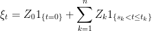
Recall that throughout these notes, we work with respect to a complete filtered probability space  . To recap, elementary predictable processes are of the form
 |
(1) |
for an  -measurable random variable
  , real numbers
  and
and  -measurable random variables
  . The integral with respect to any other process X up to time t can be written out explicitly as,
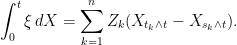 |
(2) |
The predictable sigma algebra,  , on
, on  is generated by the set of left-continuous and adapted processes or, equivalently, by the elementary predictable process. The idea behind stochastic integration is to extend this to all bounded and predictable integrands
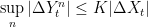
  . Other than agreeing with (2) for elementary integrands, the only other property required is bounded convergence in probability. That is, if
  is a sequence uniformly bounded by some constant K, so that
  , and converging to a limit
  then,
then,  in probability. Nothing else is required. Other properties, such as linearity of the integral with respect to the integrand follow from this, as was previously noted. Note that we are considering two random variables to be the same if they are almost surely equal. Similarly, uniqueness of the stochastic integral means that, for each integrand, the integral is uniquely defined up to probability one.
Using the definition of a semimartingale as a cadlag adapted process with respect to which the stochastic integral is well defined for bounded and predictable integrands, the main result is as follows. To be clear, in this post all stochastic processes are real-valued.
Theorem 1 A cadlag adapted process X is a semimartingale if and only if, for each  , the set
 |
(3) |
is bounded in probability.
Continue reading “Existence of the Stochastic Integral” →

is a local submartingale (resp., local supermartingale).


for some
and
.
 , is said to converge to a process X under the
  should tend to
  in probability. Also, for every sequence
  of
of  ,
,
 .
. for some
  if and only if there is a sequence
  .
.  for its closure under the semimartingale topology, the statement of the theorem is equivalent to
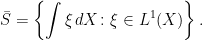
 is said to be integrable if the random variables
  are integrable, so that
 ![{{\mathbb E}[\vert X_t\vert]<\infty}](https://s0.wp.com/latex.php?latex=%7B%7B%5Cmathbb+E%7D%5B%5Cvert+X_t%5Cvert%5D%3C%5Cinfty%7D&bg=ffffff&fg=000000&s=0&c=20201002) .
.![\displaystyle X_s={\mathbb E}[X_t\mid\mathcal{F}_s]](https://s0.wp.com/latex.php?latex=%5Cdisplaystyle++X_s%3D%7B%5Cmathbb+E%7D%5BX_t%5Cmid%5Cmathcal%7BF%7D_s%5D+&bg=ffffff&fg=000000&s=0&c=20201002)
 .
. 