
A sequence of stochastic processes, 


 |
in probability for all times t. For short, this will be denoted by 
The semimartingale topology is particularly well suited to the class of semimartingales, and to stochastic integration. Previously, it was shown that the cadlag and adapted processes are complete under semimartingale convergence. In this post, it will be shown that the set of semimartingales is also complete. That is, if a sequence
Theorem 1 The space of semimartingales is complete under the semimartingale topology.
The same is true of the space of stochastic integrals defined with respect to any given semimartingale. In fact, for a semimartingale X, the set of all processes which can be expressed as a stochastic integral 
Theorem 2 Let X be a semimartingale. Then, a process Y is of the form
for some
if and only if there is a sequence
.
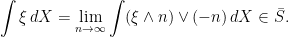
Writing S for the set of processes of the form 

 |
(1) |
Recall that the semimartingale topology is generated by a translation invariant metric 
-
.
-
for all real numbers
.
To verify that such a semimetric generates a vector topology, so that addition of processes and multiplication by scalars is continuous, the only other required property is that 

Theorem 3 A cadlag adapted process X is a semimartingale if and only if
for all sequences of real numbers
Proof: The condition that 

It follows that the semimartingales form a topological vector space.
Corollary 4 Semimartingale convergence is a vector topology on the space of semimartingales.
We now move on to the proofs of the completeness theorems. The starting point is to show that every bounded predictable integrand can be approximated by bounded elementary integrands in the following sense.
Lemma 5 Let X be a semimartingale and
for some constant K. Then, there is a sequence of elementary processes
and such that
.
Proof: Let S be the set of processes of the form
Let A be the set of predictable processes 

 |
So, 
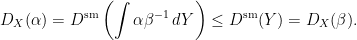
Next, stochastic integration of a bounded predictable process is a Lipschitz continuous map on the semimartingales.
Lemma 6 Let
be a constant and
.
If, furthermore, X is a semimartingale then this holds for all predictable
Proof: Recall that 

![\displaystyle {\mathbb E}\left[\left\vert \alpha_0X_0+\int_0^t\alpha\,dX\right\vert\wedge 1\right]](https://s0.wp.com/latex.php?latex=%5Cdisplaystyle++%7B%5Cmathbb+E%7D%5Cleft%5B%5Cleft%5Cvert+%5Calpha_0X_0%2B%5Cint_0%5Et%5Calpha%5C%2CdX%5Cright%5Cvert%5Cwedge+1%5Cright%5D+&bg=ffffff&fg=000000&s=0&c=20201002) |
over all elementary 


![\displaystyle \setlength\arraycolsep{2pt} \begin{array}{rl} \displaystyle{\mathbb E}\left[\left\vert\int_0^t\alpha\,dY\right\vert\wedge 1\right] &\displaystyle= {\mathbb E}\left[\left\vert\int_0^t\alpha\xi\,dX\right\vert\wedge 1\right]\smallskip\\ &\displaystyle\le K{\mathbb E}\left[\left\vert\int_0^t K^{-1}\alpha\xi\,dX\right\vert\wedge 1\right]\smallskip\\ &\displaystyle\le K D^{\rm sm}_t(X). \end{array}](https://s0.wp.com/latex.php?latex=%5Cdisplaystyle++%5Csetlength%5Carraycolsep%7B2pt%7D+%5Cbegin%7Barray%7D%7Brl%7D+%5Cdisplaystyle%7B%5Cmathbb+E%7D%5Cleft%5B%5Cleft%5Cvert%5Cint_0%5Et%5Calpha%5C%2CdY%5Cright%5Cvert%5Cwedge+1%5Cright%5D+%26%5Cdisplaystyle%3D+%7B%5Cmathbb+E%7D%5Cleft%5B%5Cleft%5Cvert%5Cint_0%5Et%5Calpha%5Cxi%5C%2CdX%5Cright%5Cvert%5Cwedge+1%5Cright%5D%5Csmallskip%5C%5C+%26%5Cdisplaystyle%5Cle+K%7B%5Cmathbb+E%7D%5Cleft%5B%5Cleft%5Cvert%5Cint_0%5Et+K%5E%7B-1%7D%5Calpha%5Cxi%5C%2CdX%5Cright%5Cvert%5Cwedge+1%5Cright%5D%5Csmallskip%5C%5C+%26%5Cdisplaystyle%5Cle+K+D%5E%7B%5Crm+sm%7D_t%28X%29.+%5Cend%7Barray%7D+&bg=ffffff&fg=000000&s=0&c=20201002) |
Taking the supremum over all such 
Now suppose that X is a semimartingale and 
 |
⬜
The proof of Theorem 1 for the completeness of the space of semimartingales is as follows.
Theorem 7 Let
Proof: According to the definition of semimartingales used in these notes, it needs to be shown that there is a well-defined stochastic integral with respect to X for bounded integrands which agrees with the explicit expression for elementary integrands and satisfies bounded convergence in probability.
Using the semimartingale topology, Lemma 6 says that, for any bounded elementary 
 |
(2) |
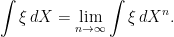
If 
Now suppose that 

For the remainder of the post, let us turn our attention towards the proof of Theorem 2. If S is the set of integrals
 |
(3) |
which is established by the following lemma.
Lemma 8 Let X be a semimartingale and
.
Proof: This is stated by Lemma 5 in the case where
 |
⬜
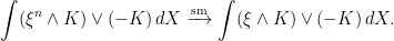
Proving the reverse inclusion to (3) is more difficult. By definition, for any 

For convenience, the notation 


 |
(4) |
The following will be used to show that certain sums of predictable processes converge absolutely to an X-integrable process.
Lemma 9 Let X be a semimartingale and
be a sequence of bounded predictable processes with
. Setting
then, for each t,
(5) is bounded in probability. Furthermore, if
is a sequence of bounded predictable processes with
then
.
Proof: Setting 

 |
So, for constant 
 |
The inequality here is just the triangle inequality combined with (4). It follows that if 


 |
Here, the terms inside the summation are bounded by 


Next, the sum 
Lemma 10 Let X and
is predictable and
for all bounded predictable

Proof: The fact that A is predictable follows from the condition that 


Finally, the reverse inclusion to (3) can be shown, completing the proof of Theorem 2.
Lemma 11 Let X be a semimartingale, S be the set of integrals
Proof: By definition, for any 
Then, set 
 |
is finite. So, setting 


 |
As 
 |
Finally, Lemma 10 gives 
 |
as required. ⬜
Notes
Completeness of the set of stochastic integrals with respect to a semimartingale was originally stated by Memin, in the paper Espaces de semi martingales et changement de probabilité. This uses quite different techniques to those employed in this post. In Memin’s approach, stochastic integration was defined with respect to decompositions into local martingale and finite variation terms. Completeness of stochastic integrals for the local martingale and finite variation components can be inferred from completeness of 

The link to the monotone class theorem on planetmath is broken; the correct link is http://planetmath.org/functionalmonotoneclasstheorem.
Thanks for your great blog!
Fixed (eventually…). Thanks!
This now links to my own post on the monotone class theorem: https://almostsure.wordpress.com/2019/10/27/the-functional-monotone-class-theorem