Predictable Stopping Times

The concept of a stopping times was introduced a couple of posts back. Roughly speaking, these are times for which it is possible to observe when they occur. Often, however, it is useful to distinguish between different types of stopping times. A random time for which it is possible to predict when it is about to occur is called a predictable stopping time. As always, we work with respect to a filtered probability space ${(\Omega,\mathcal{F},\{\mathcal{F}_t\}_{t\ge 0},{\mathbb P})}$ .

Definition 1 A map ${\tau\colon\Omega\rightarrow\bar{\mathbb R}_+}$ is a predictable stopping time if there exists a sequence of stopping times ${\tau_n\uparrow\tau}$ satisfying ${\tau_n<\tau}$ whenever ${\tau\not=0}$ .

Predictable stopping times are alternatively referred to as previsible. The sequence of times ${\tau_n}$ in this definition are said to announce ${\tau}$ . Note that, in this definition, the random time was not explicitly required to be a stopping time. However, this is automatically the case, as the following equation shows.

$\displaystyle \left\{\tau\le t\right\}=\bigcap_n\left\{\tau_n\le t\right\}\in\mathcal{F}_t.$

One way in which predictable stopping times occur is as hitting times of a continuous adapted process. It is easy to predict when such a process is about to hit any level, because it must continuously approach that value.

Theorem 2 Let ${X}$ be a continuous adapted process and ${K}$ be a real number. Then

$\displaystyle \tau=\inf\left\{t\in{\mathbb R}_+\colon X_t\ge K\right\}$

is a predictable stopping time.

Proof: Let ${\tau_n}$ be the first time at which ${X_t\ge K-1/n}$ which, by the debut theorem, is a stopping time. This gives an increasing sequence bounded above by ${\tau}$ . Also, ${X_{\tau_n}\ge K-1/n}$ whenever ${\tau_n<\infty}$ and, by left-continuity, setting ${\sigma=\lim_n\tau_n}$ gives ${X_\sigma\ge K}$ whenever ${\sigma<\infty}$ . So, ${\sigma\ge\tau}$ , showing that the sequence ${\tau_n}$ increases to ${\tau}$ . If ${0<\tau_n\le\tau<\infty}$ then, by continuity, ${X_{\tau_n}=K-1/n\not=K=X_{\tau}}$ . So, ${\tau_n<\tau}$ whenever ${0<\tau<\infty}$ and the sequence ${n\wedge\tau_n}$ announces ${\tau}$ . ⬜

In fact, predictable stopping times are always hitting times of continuous processes, as stated by the following result. Furthermore, by the second condition below, it is enough to prove the much weaker condition that a random time can be announced `in probability’ to conclude that it is a predictable stopping time.

Lemma 3 Suppose that the filtration is complete and ${\tau\colon\Omega\rightarrow\bar{\mathbb R}_+}$ is a random time. The following are equivalent.

${\tau}$ is a predictable stopping time.

For any ${\epsilon,\delta,K>0}$ there is a stopping time ${\sigma}$ satisfying

$\displaystyle {\mathbb P}\left(K\wedge\tau-\epsilon<\sigma<\tau{\rm\ or\ }\sigma=\tau=0\right)>1-\delta.$ (1)

${\tau=\inf\{t\ge 0\colon X_t=0\}}$ for some continuous adapted process ${X}$ .

Proof: If ${\tau}$ is predictable then there is a sequence ${\tau_n}$ of stopping times announcing ${\tau}$ . This means that ${K\wedge\tau-\epsilon<\tau_n<\tau}$ or ${\tau_n=\tau=0}$ for large ${n}$ . By bounded convergence, (1) is satisfied with ${\sigma=\tau_n}$ and large ${n}$ .

Now suppose that the second statement holds. In order to construct the process ${X}$ satisfying the third condition, it is enough to find an adapted continuous process ${Y_t}$ taking values in ${\bar{\mathbb R}_+}$ , and which is finite for ${t<\tau}$ and infinite for ${t\ge\tau}$ . Then, ${X}$ can be obtained by ${X_t=1/(1+Y_t)}$ . Furthermore, ${X_t}$ can be replaced by ${\tau-t}$ on any zero probability set and, by completeness of the filtration, it will still be adapted. So, ${Y}$ only has to have the above properties with probability one.

By equation (1), there is a sequence ${\tau_n}$ of stopping times satisfying

$\displaystyle {\mathbb P}(n\wedge\tau-2^{-n}<\tau_n<\tau{\rm\ or\ }\tau_n=\tau=0)>1-2^{-n}.$

(2)

The Borel-Cantelli lemma shows that, with probability one, ${n\wedge\tau-2^{-n}<\tau_n<\tau}$ or ${\tau_n=\tau=0}$ for all large ${n}$ . In particular, ${\{\tau=0\}}$ equals ${\{\tau_n=0{\rm\ infinitely\ often}\}}$ up to a zero probability set, so is ${\mathcal{F}_0}$ -measurable. Choosing a sequence of positive reals ${\lambda_n}$ , set ${Y_t=\infty}$ on the set ${\tau=0}$ and

$\displaystyle Y_t = \sum_{n=1}^\infty \lambda_n\max(t-\tau_n,0)$

otherwise. As ${\tau_n\rightarrow\tau}$ , this reduces to a finite sum when ${t<\tau}$ . It only remains to show that for large enough ${\lambda_n}$ , the left limit at ${\tau}$

$\displaystyle Y_{\tau-}=\sum_{n=1}^\infty \lambda_n\max(\tau-\tau_n,0),$

will be almost surely infinite whenever ${\tau>0}$ . By monotone convergence, equation (2) gives ${{\mathbb P}(\lambda_n(\tau-\tau_n)<1{\rm\ and\ }\tau>0)<2^{-n}}$ for large ${\lambda_n}$ . In this case, another application of the Borel-Cantelli lemma gives, with probability one, ${\lambda_n(\tau-\tau_n)\ge 1}$ for all large ${n}$ when ${\tau>0}$ , so ${Y_{\tau-}}$ is indeed infinite.

Finally, using Theorem 2, the first statement follows from the second. ⬜

As with general stopping times, the class of predictable stopping times is closed under basic operations such as taking the maximum and minimum of two times.

Lemma 4 If ${\sigma,\tau}$ are predictable stopping times, then so are ${\sigma\wedge\tau,\sigma\vee\tau}$ .

Proof: If ${\sigma_n,\tau_n}$ announce ${\sigma}$ and ${\tau}$ then it is clear that ${\sigma_n\wedge\tau_n}$ and ${\sigma_n\vee\tau_n}$ announce ${\sigma\wedge\tau}$ and ${\sigma\vee\tau}$ respectively. ⬜

Furthermore, the predictable stopping times are closed under taking limits of sequences, under some conditions. For example, increasing sequences or eventually constant sequences of predictable stopping times are predictable.

Lemma 5 Let ${(\tau_n)_{n=1,2,\ldots}}$ be a sequence of predictable stopping times. Then,

${\tau=\sup_n\tau_n}$ is a predictable stopping time.

if there is a limit satisfying ${\tau_n(\omega)=\tau(\omega)}$ eventually (for all ${\omega}$ ), and the filtration is complete, then ${\tau}$ is a predictable stopping time.

Proof: Let ${(\tau_{nm})_{m=1,2,\ldots}}$ announce ${\tau_n}$ . For the first statement, the sequence ${\sigma_n\equiv\max\{\tau_{jk}\colon j,k\le n\}}$ announces ${\tau}$ .

For the second statement, choose any ${\epsilon,\delta,K>0}$ and ${n}$ large enough such that ${{\mathbb P}(\tau_n\not=\tau)<\delta/2}$ . By Lemma 3, there is a stopping time ${\sigma}$ satisfying

$\displaystyle {\mathbb P}(K\wedge\tau_n-2^{-n}<\sigma<\tau_n{\rm\ or\ }\sigma=\tau_n=0)>1-\delta/2.$

It follows that equation (1) is satisfied and, by Lemma 3, ${\tau}$ is predictable. ⬜

As shown in the previous post, given a stopping time ${\tau}$ and a set ${A\in\mathcal{F}_\tau}$ , the time ${\tau_A}$ as defined below will also be a stopping time.

$\displaystyle \tau_A(\omega)\equiv\begin{cases} \tau(\omega),&\textrm{if }\omega\in A,\\ \infty,&\textrm{otherwise} \end{cases}$

(3)

If, however, ${\tau}$ is a predictable stopping time then ${\tau_A}$ need not be predictable. For this to be true, we need to restrict the set ${A}$ to be in ${\mathcal{F}_{\tau-}}$ .

Lemma 6 Suppose that the filtration is complete. If ${\tau}$ is a predictable stopping time and ${A\in\mathcal{F}_{\tau-}}$ , then ${\tau_A}$ is a predictable stopping time.

Proof: Let ${\tau_n}$ be stopping times announcing ${\tau}$ and set ${\mathcal{G}=\bigcup_n\mathcal{F}_{\tau_n}}$ . As proven in the previous post, ${\mathcal{F}_{\tau-}=\sigma(\mathcal{G})}$ . The monotone class theorem shows that for any ${\delta>0}$ there is a set ${B\in\mathcal{G}}$ with ${{\mathbb E}[|1_A-1_B|]<\delta}$ .

Then, ${B\in\mathcal{F}_{\tau_n}}$ for large ${n}$ so, as shown in the previous post, ${(\tau_n)_B}$ will be a stopping time. For any ${\epsilon,\delta,K>0}$ ,

$\displaystyle \setlength\arraycolsep{2pt} \begin{array}{rcl} &&\displaystyle{\mathbb P}(K\wedge\tau_A<(\tau_n)_B<\tau_A{\rm\ or\ }(\tau_n)_B=\tau_A=0)\smallskip\\ &\displaystyle\ge&\displaystyle{\mathbb P}(K\wedge\tau_A<(\tau_n)_A<\tau_A{\rm\ or\ }(\tau_n)_A=\tau_A=0)-{\mathbb P}((\tau_n)_B\not=(\tau_n)_A)\smallskip\\ &\displaystyle\ge&\displaystyle{\mathbb P}(K\wedge\tau<\tau_n<\tau{\rm\ or\ }\tau_n=\tau=0)-{\mathbb E}[|1_A-1_B|] \end{array}$

which, by bounded convergence, is greater than ${1-\delta}$ for large ${n}$ . Lemma 3 completes the proof. ⬜

Predictable stopping times are sometimes used to define the predictable sigma-algebra. In these notes, it was defined as the sigma-algebra generated by the adapted and left-continuous (or, just continuous) processes, which is a bit more direct. However, an alternative definition is that it is the sigma-algebra generated by the stochastic intervals ${[\tau,\infty)}$ for predictable stopping times ${\tau}$ . A stochastic interval is a `random interval’ of the real numbers, whose endpoints are random variables. This expresses a subset of ${{\mathbb R}_+\times\Omega}$ ,

$\displaystyle [\tau,\infty)\equiv\left\{(t,\omega)\in {\mathbb R}_+\times\Omega\colon \tau(\omega)\le t\right\}.$

Similarly, the optional sigma-algebra can also be generated by such intervals, where ${\tau}$ is an arbitrary stopping time, not necessarily predictable. However, optional processes are not used in these notes beyond the definition in the first few posts, so we do not prove that here.

Lemma 7 The predictable sigma algebra is

$\displaystyle \mathcal{P}=\sigma\left(\{[\tau,\infty)\colon \tau{\rm\ is\ a\ predictable\ stopping\ time}\}\right).$

Proof: If ${\tau_n}$ is a sequence of stopping times announcing ${\tau}$ , then ${X^n_t=1_{\{t>\tau_n{\rm\ or\ }\tau_n=0\}}}$ are adapted left-continuous and hence predictable processes. So,

$\displaystyle [\tau,\infty)=\bigcap_n\left((\tau_n,\infty)\cup({\mathbb R}_+\times\{\tau_n=0\})\right)\in\mathcal{P}$

So, the collection ${\mathcal{G}}$ of sets of the form ${[\tau,\infty)}$ for predictable stopping times ${\tau}$ is contained in the predictable sigma-algebra. Conversely, ${\mathcal{P}}$ is generated by the following sets

${S={\mathbb R}_+\times A}$ for ${A\in\mathcal{F}_0}$ . Letting ${\tau}$ be the identically zero stopping time, this is ${[\tau_A,\infty)\in\mathcal{G}}$ .
${S=(t,\infty)\times A}$ for ${A\in\mathcal{F}_t}$ . Letting ${\tau_n}$ be the stopping time identically equal to ${t+1/n}$ shows that ${S=\bigcap_n[(\tau_n)_A,\infty)}$ is in the sigma-algebra generated by ${\mathcal{G}}$ .

So, ${\mathcal{P}}$ is contained in, and hence equals, ${\sigma(\mathcal{G})}$ . ⬜

Finally, it is useful to realize that the set of predictable stopping times is almost the same, regardless of whether it is defined with respect to the filtration ${\mathcal{F}_t}$ or the right-continuous filtration ${\mathcal{F}_{t+}}$ . Many approaches to stochastic calculus assume that the filtration satisfies `usual conditions’ and, in particular, is right-continuous. However, the results can often be directly carried across to the more general situation simply by applying them to the right-continuous filtration ${\mathcal{F}_{t+}}$ .

Lemma 8 A random time ${\tau}$ is a predictable stopping time if and only if it is a predictable stopping time with respect to the right-continuous filtration ${\mathcal{F}_{t+}}$ and ${\{\tau=0\}\in\mathcal{F}_0}$ .

Proof: Any predictable stopping time is still clearly a predictable stopping time under the larger filtration ${\mathcal{F}_{t+}}$ , so only the converse needs to be proven. However, in this case, Lemma 3 shows that ${\tau}$ is the first time at which some continuous and ${\mathcal{F}_{t+}}$ -adapted process ${X}$ hits zero. Multiplying by ${1_{\{\tau>0\}}/X_0}$ if necessary, this process can be assumed to satisfy ${X_0=1_{\{\tau=0\}}}$ , which is ${\mathcal{F}_0}$ -measurable. Furthermore, by left-continuity, ${X_t}$ will in fact be ${\mathcal{F}_{t-}}$ -measurable at each positive time, so it is adapted. The result now follows from Theorem 2. ⬜

Accessible and inaccessible times

The flip side of the coin to predictable stopping times are totally inaccessible stopping times. These are times which cannot be predicted with any positive probability. Simple examples include the jump times of a Poisson process.

Definition 9 A stopping time ${\tau}$ is

totally inaccessible if ${{\mathbb P}(\sigma=\tau<\infty)=0}$ for all predictable stopping times ${\sigma}$ .

accessible if there exists a sequence of predictable stopping times ${\tau_n}$ such that
$\displaystyle \tau(\omega)\in\left\{\tau_1(\omega),\tau_2(\omega),\ldots\right\}$

for all ${\omega}$ .

The graph ${[\tau]}$ of a random time is the set ${\{(\tau(\omega),\omega)\colon\omega\in\Omega,\tau(\omega) < \infty\}}$ , so a stopping time is accessible if its graph is contained in the graphs of a countable set of predictable stopping times. Accessible and totally inaccessible stopping times are always disjoint in the following sense. If ${\sigma}$ is accessible and ${\tau}$ is totally inaccessible then ${{\mathbb P}(\sigma=\tau<\infty)=0}$ . This follows directly from the definition above.

Arbitrary stopping times have a unique decomposition into their accessible and totally inaccessible parts. Actually, the proof below doesn’t make any use if the properties of predictable stopping times, and will still work if the term `predictable stopping time’ is replaced by any other type of stopping time.

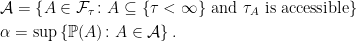
Theorem 10 If ${\tau}$ is a stopping time, then there exists an ${A\subseteq\{\tau<\infty\}}$ such that ${\tau_A}$ (defined by equation 3) is an accessible stopping time and ${\tau_{A^c}}$ is a totally inaccessible stopping time.

Furthermore, ${A}$ is uniquely defined up to a set of zero probability.

Proof: First, as ${\tau_A}$ is a stopping time, ${A\cap\{\tau\le t\}=\{\tau_A\le t\}\in\mathcal{F}_t}$ , so it is necessarily true that ${A\in\mathcal{F}_\tau}$ . Set

$\displaystyle \setlength\arraycolsep{2pt} \begin{array}{rl} &\displaystyle\mathcal{A}=\left\{A\in\mathcal{F}_\tau\colon A\subseteq\{\tau<\infty\}{\rm\ and\ }\tau_A{\rm\ is\ accessible}\right\}\smallskip\\ &\displaystyle\alpha=\sup\left\{{\mathbb P}(A)\colon A\in\mathcal{A}\right\}. \end{array}$

If ${A_n\in\mathcal{A}}$ is any sequence and ${A=\bigcup_nA_n}$ , then the graph of ${\tau_A}$ is contained in the union of the graphs of ${\tau_{A_n}}$ which, in turn, are each contained in the graphs of countable sets of predictable stopping times. As countable unions of countable sets are themselves countable, it follows that ${\tau_A}$ is accessible. So, ${\mathcal{A}}$ is closed under countable unions. In particular, choosing ${A_n}$ such that ${{\mathbb P}(A_n)\rightarrow\alpha}$ gives ${{\mathbb P}(A)\ge\alpha}$ . Therefore, there is an ${A\in\mathcal{A}}$ with ${{\mathbb P}(A)=\alpha}$ .

For ${A\in\mathcal{A}}$ , the next step is to show that ${\tau_{A^c}}$ is totally inaccessible if and only if ${{\mathbb P}(A)=\alpha}$ . First, if ${{\mathbb P}(A)=\alpha}$ and ${\sigma}$ is a predictable stopping time then ${B=A\cup\{\sigma=\tau<\infty\}}$ is in ${\mathcal{A}}$ and ${{\mathbb P}(B)=\alpha+{\mathbb P}(\sigma=\tau_{A^c}<\infty)}$ . From the definition of ${\alpha}$ , this gives ${{\mathbb P}(\sigma=\tau_{A^c}<\infty)=0}$ and ${\tau_{A^c}}$ is totally inaccessible. Conversely, let ${\tau_{A^c}}$ be totally inaccessible. For any ${B\in\mathcal{A}}$ , ${{\mathbb P}(\tau_{A^c}=\tau_B<\infty)=0}$ and, therefore, ${{\mathbb P}(B\setminus A)=0}$ and, consequently, ${{\mathbb P}(A)\ge{\mathbb P}(B)}$ . So, ${{\mathbb P}(A)=\alpha}$ .

This shows that there is an ${A\in\mathcal{A}}$ satisfying ${{\mathbb P}(A)=\alpha}$ , which then satisfies the conclusion of the lemma. Finally, if there is a ${B}$ also satisfying the required properties, then so do ${A\cup B}$ and ${A\cap B}$ . This gives ${{\mathbb P}(A\cup B)={\mathbb P}(A\cap B)=\alpha}$ and ${A,B}$ differ by a zero probability set. ⬜

Thin sets and jump times of a process

Stopping times are often used to control what happens when a process jumps. As we shall see, the set of jump times of a càdlàg adapted process can be covered by a sequence of stopping times and, furthermore, can be decomposed into predictable and totally inaccessible times. To state this in slightly more generality, we start with the definition of thin sets, the standard example being the set of jump times of an adapted process.

Definition 11 A set ${A\subseteq{\mathbb R}_+\times\Omega}$ is said to be a thin set if ${A=\bigcup_{n=1}^\infty[\tau_n]}$ for a sequence of stopping times ${\tau_n}$ .

A process X is said to be thin if it is optional and

$\displaystyle \{X\not=0\}\equiv\{(t,\omega)\in{\mathbb R}_+\times\Omega\colon X_t(\omega)\not=0\}$

is a thin set.

So, countable unions of thin sets are thin. Also, every progressively measurable subset and, in particular, every optional subset of a thin set is itself thin.

Lemma 12 If A is a thin set then any progressively measurable subset of A is thin.

Proof: Suppose that ${A=\bigcup_n[\tau_n]}$ for stopping times ${\tau_n}$ and ${B\subseteq A}$ is progressive. Set ${B_n=\{\omega\in\Omega\colon(\tau_n(\omega),\omega)\in B\}}$ . As ${1_{B_n}}$ is the value of the progressively measurable process ${1_B}$ at time ${\tau_n}$ , we have ${B_n\in\mathcal{F}_{\tau_n}}$ . So, ${(\tau_n)_{B_n}}$ are stopping times and

$\displaystyle B=\bigcup_{n=1}^\infty[(\tau_n)_{B_n}]$

is thin. ⬜

For example, if X and Y are thin processes then this shows that the sum ${X+Y}$ is also thin. Being the sum of optional processes, ${X+Y}$ will be optional and, ${\{X+Y\not=0\}\subseteq\{X\not=0\}\cup\{Y\not=0\}}$ is thin.

As mentioned above, thin sets are often used to represent the set of jump times of a process. For the concept of the jumps of a process X to make sense, it is necessary to apply some constraints on its sample paths. We suppose that ${t\mapsto X_t}$ is right-continuous with left limits everywhere. Such processes are called càdlàg from the French “continu à droite, limites à gauche”. Alternatively, they are sometimes known as rcll processes (right-continuous with left limits). The left limit at any time ${t > 0}$ is denoted by ${X_{t-}}$ , and we set ${X_{0-}=X_0}$ . Then, ${X_-}$ is a left-continuous process. The jumps of X are denoted by ${\Delta X_t=X_t-X_{t-}}$ .

Lemma 13 If X is a càdlàg adapted process then ${\Delta X}$ is thin.

Proof: First, as ${X,X_-}$ are adapted and respectively right and left-continuous, they are progressive. So, ${\Delta X=X-X_-}$ is progressive. For each ${s,a\in{\mathbb Q}_+}$ define the stopping time

$\displaystyle \tau_{s,a}=\inf\left\{t\ge s\colon\vert X_t-X_s\vert\ge a\right\}.$

Consider any sample path of X and time t such that ${\Delta X_t\not=0}$ . For any positive rational ${a < \vert\Delta X\vert/2}$ , the existence of left limits along the sample path implies the existence of a positive rational ${s < t}$ such that ${\vert X_u-X_s\vert < a}$ for all u in the interval ${(s,t)}$ . It can be seen that ${\tau_{s,a}=t}$ . So,

$\displaystyle \{\Delta X\not=0\}\subseteq \bigcup_{s,a\in{\mathbb Q}_+}[\tau_{s,a}]$

is thin. ⬜

We shall refer to a thin set A as accessible if every stopping time ${\tau}$ satisfying ${[\tau]\subseteq A}$ is accessible. Similarly, we shall refer to A as totally inaccessible if every such stopping time is totally inaccessible. Then the collection of accessible (respectively, totally inaccessible) thin sets is closed under taking countable unions and progressively measurable subsets. Note that if A is both accessible and totally inaccessible then every stopping time ${[\tau]\subseteq A}$ is both accessible and totally inaccessible, so ${{\mathbb P}(\tau < \infty)=0}$ . Therefore, A is evanescent. Similarly, if A is accessible and B is totally inaccessible then ${A\cap B}$ is evanescent.

Theorem 10 above generalises to give a decomposition of thin sets into their accessible and totally inaccessible parts.

Theorem 14 Let A be a thin set. Then, up to evanescence, there is a unique decomposition into thin sets ${A=B\cup C}$ , where B is accessible and C is totally inaccessible.

Proof: Write ${A=\bigcup_n[\tau_n]}$ for a sequence of stopping times ${\tau_n}$ . By Theorem 10 there are sets ${A_n\in\mathcal{F}_{\tau_n}}$ such that ${(\tau_n)_{A_n}}$ are accessible stopping times and ${(\tau_n)_{A_n^c}}$ are totally inaccessible. The required decomposition ${A=B\cup C}$ is given by

$\displaystyle B=\bigcup_{n=1}^\infty[(\tau_n)_{A_n}],\ C=\bigcup_{n=1}^\infty[(\tau_n)_{A_n^c}].$

Suppose that ${A=B^\prime\cup C^\prime}$ is any other such decomposition. Then,

$\displaystyle B^\prime=A\cap B^\prime=(B\cap B^\prime)\cup(C\cap B^\prime).$

However, ${C\cap B^\prime}$ is evanescent. So, ${B^\prime\subseteq B}$ up to evanescence. Combining this with the reverse inclusion gives ${B^\prime=B}$ and ${C^\prime=C}$ up to evanescence. ⬜

We finally show that every thin set is contained in the disjoint graphs of a sequence of stopping times, each of which is either predictable or totally inaccessible. This can be useful when looking at the jumps of a process to break the problem down into the separate cases of predictable jump times and totally inaccessible jump times.

Theorem 15 Suppose that the filtration is complete and that ${A\subseteq{\mathbb R}_+\times\Omega}$ is a thin set. Then ${A\subseteq\bigcup_{n=1}^\infty[\tau_n]}$ for a sequence of stopping times ${\tau_n}$ satisfying,

For each n, ${\tau_n}$ is either predictable or totally inaccessible.

For each ${m\not=n}$ we have ${\tau_m\not=\tau_n}$ whenever ${\tau_n < \infty}$ .

Proof: First, by definition, there is a sequence ${\sigma_n}$ of stopping times such that ${A=\bigcup_n[\sigma_n]}$ . For each n define the set

$\displaystyle A_n=\left\{\omega\in\Omega\colon\sigma_n(\omega)\not\in\{\sigma_1(\omega),\ldots,\sigma_{n-1}(\omega)\}\right\}.$

(4)

As ${1_{A_n}}$ is just the value of the optional process ${1-1_{[\sigma_1]\cup\cdots\cup[\sigma_{n-1}]}}$ at time ${\sigma_n}$ we have ${A_n\in\mathcal{F}_{\tau_n}}$ . So, ${\tau_n=(\sigma_n)_{A_n}}$ are stopping times with

$\displaystyle A=\bigcup_{n=1}^\infty[\sigma_n]=\bigcup_{n=1}^\infty[\tau_n].$

Also, by construction, we have ${\omega\in A_n}$ whenever ${\tau_n(\omega) < \infty}$ and, hence, ${\tau_n(\omega)\not=\tau_m(\omega)}$ for each ${m < n}$ as required. It only remains to be shown that the stopping times ${\tau_n}$ can each be chosen to be either predictable or totally inaccessible.

Consider the case where A is accessible. By definition, writing ${A=\bigcup_n[\sigma^0_n]}$ for stopping times ${\sigma^0_n}$ , we have that ${\sigma^0_n}$ are accessible. So, there is a doubly-indexed sequence of predictable times ${\sigma_{n,m}}$ with ${[\sigma^0_n]\subseteq\bigcup_m[\sigma_{n,m}]}$ . Reindexing the sequence ${\sigma_{m,n}}$ gives a sequence ${\sigma_1,\sigma_2,\ldots}$ of predictable stopping times such that the thin set ${A^\prime\equiv\bigcup_n[\sigma_n]}$ contains A. Now apply the argument above to ${A^\prime}$ . The set ${A_n}$ defined by (4) is in ${\mathcal{F}_{\sigma_n-}}$ , since ${1_{A_n}}$ is the value of the predictable process ${1-1_{[\sigma_1]\cup\cdots\cup[\sigma_{n-1}]}}$ at time ${\sigma_n}$ . By Lemma 6 (which requires completeness of the filtration), the times ${\tau_n=(\sigma_n)_{A_n}}$ are predictable. This proves the result in the case where A is accessible.

Finally, consider any thin set A. By Theorem 14 we can decompose ${A=B\cup C}$ for B accessible and C totally inaccessible. As shown above, the result can be applied to the accessible set B to get predictable stopping times ${\tau^1_n}$ such that ${B\subseteq\bigcup_n[\tau^1_n]}$ and ${\tau^1_m\not=\tau^1_n}$ whenever ${m\not=n}$ and ${\tau^1_n < \infty}$ . Then apply the argument above to the thin set ${C^\prime\equiv C\setminus\bigcup_n[\tau^1_n]}$ to obtain stopping times ${\tau^2_n}$ with ${C^\prime=\bigcup_n[\tau^2_n]}$ and ${\tau^2_m\not=\tau^2_n}$ whenever ${m\not=n}$ and ${\tau^2_n < \infty}$ .

We have constructed predictable stopping times ${\tau^1_n}$ and stopping times ${\tau^2_n}$ . The graphs ${[\tau^1_n],[\tau^2_n]}$ ( ${n\in{\mathbb N}}$ ) are all disjoint and have union containing A. Furthermore, as ${[\tau^2_n]}$ are all contained in C, ${\tau^2_n}$ are totally inaccessible times. The result now follows by merging the sequences ${\tau^1_n}$ and ${\tau^2_n}$ together into a single sequence. ⬜

7 thoughts on “Predictable Stopping Times”

George Lowther says:

3 November 11 at 12:53 AM

Update: I added an extra section to this post. This introduces the notion of thin sets, and shows that the collection of jump times of a cadlag process can be covered by a sequence of stopping times, each of which is predictable or totally inaccessible. These are very simple ideas, but very useful, especially in some of the `general theory’ which I have been writing recently.

Anonymous says:

5 September 12 at 10:40 PM

Hi. I like your blog and learnt a lot. I have a question related to this topic. Since the predictable sigma field is contained in the optional sigma field generated by rcll processes, a predictable process is an optional process. My question is: when a rcll process is a predictable process?

1. George Lowther says:
  
  6 September 12 at 2:36 AM
  
  Hi. Actually I wrote out a lemma in a later post answering precisely this question (link).
  
Dominic says:

10 December 12 at 3:39 AM

Hi, I’m a little confused how you got the second inequality in Lemma 6. It seems to me that the event in the second line implies the event in the third (giving an inequality in the opposite direction), but hopefully I’m mistaken here.

Pingback: Proof of Optional and Predictable Section | Almost Sure
Harvey Stein says:

2 April 19 at 9:21 PM

Thanks for the blog. Very helpful. Typo: In “If $\sigma$ is accessible and $\tau$ is totally accessible then $\mathbb P(\sigma=\tau < \infty)=0$ , the 2nd "accessible" should be "inaccessible".

1. George Lowther says:
  
  4 April 19 at 12:21 AM
  
  Fixed. Thanks

	Tavin on Class (D) Processes
	George Lowther on Filtrations and Adapted P…
	faceet on Filtrations and Adapted P…
	George Lowther on Filtrations and Adapted P…
	facet on Filtrations and Adapted P…
	Zoltan on Class (D) Processes
	Zoltan on Class (D) Processes
	ARS on Stopping Times and the Debut…
	George Lowther on Upcrossings, Downcrossings, an…
	George Lowther on Stopping Times and the Debut…

Predictable Stopping Times

Accessible and inaccessible times

Thin sets and jump times of a process

Published by George Lowther

7 thoughts on “Predictable Stopping Times”

Leave a Reply Cancel reply

Accessible and inaccessible times

Thin sets and jump times of a process

Like this:

Related

Published by George Lowther

7 thoughts on “Predictable Stopping Times”

Leave a Reply Cancel reply