In this post I attempt to give a rigorous definition of integration with respect to Brownian motion (as introduced by Itô in 1944), while keeping it as concise as possible. The stochastic integral can also be defined for a much more general class of processes called semimartingales. However, as Brownian motion is such an important special case which can be handled directly, I start with this as the subject of this post. If  is a standard Brownian motion defined on a probability space
  and
and  is a stochastic process, the aim is to define the integral
 |
(1) |
In ordinary calculus, this can be approximated by Riemann sums, which converge for continuous integrands whenever the integrator  is of finite variation. This leads to the Riemann-Stietjes integral and, generalizing to measurable integrands, the Lebesgue-Stieltjes integral. Unfortunately this method does not work for Brownian motion which, as discussed in my previous post, has infinite variation over all nontrivial compact intervals.
The standard approach is to start by writing out the integral explicitly for piecewise constant integrands. If there are times  such that
  for each
  then the integral is given by the summation,
 |
(2) |
We could try to extend to more general integrands by approximating by piecewise constant processes but, as mentioned above, Brownian motion has infinite variation paths and this will diverge in general.
Fortunately, when working with random processes, there are a couple of observations which improve the chances of being able to consistently define the integral. They are
- The integral is not a single real number, but is instead a random variable defined on the probability space. It therefore only has to be defined up to a set of zero probability and not on every possible path of .
- Rather than requiring limits of integrals to converge for each path of (e.g., dominated convergence), the much weaker convergence in probability can be used.
These observations are still not enough, and the main insight is to only look at integrands which are adapted. That is, the value of  can only depend on through its values at prior times. This condition is met in most situations where we need to use stochastic calculus, such as with (forward) stochastic differential equations. To make this rigorous, for each time
  let
let  be the sigma-algebra generated by
  for all
  . This is a filtration (
 for ), and
  is referred to as a filtered probability space. Then,
  is adapted if is -measurable for all times
  . Piecewise constant and left-continuous processes, such as in (2), which are also adapted are commonly referred to as simple processes.
However, as with standard Lebesgue integration, we must further impose a measurability property. A stochastic process can be viewed as a map from the product space  to the real numbers, given by
  . It is said to be jointly measurable if it is measurable with respect to the product sigma-algebra
  , where
  refers to the Borel sigma-algebra. Finally, it is called progressively measurable, or just progressive, if its restriction to
 ![{[0,t]\times\Omega}](https://s0.wp.com/latex.php?latex=%7B%5B0%2Ct%5D%5Ctimes%5COmega%7D&bg=ffffff&fg=000000&s=0&c=20201002) is
is ![{\mathcal{B}([0,t])\otimes\mathcal{F}_t}](https://s0.wp.com/latex.php?latex=%7B%5Cmathcal%7BB%7D%28%5B0%2Ct%5D%29%5Cotimes%5Cmathcal%7BF%7D_t%7D&bg=ffffff&fg=000000&s=0&c=20201002) -measurable for each positive time . It is easily shown that progressively measurable processes are adapted, and the simple processes introduced above are progressive.
-measurable for each positive time . It is easily shown that progressively measurable processes are adapted, and the simple processes introduced above are progressive.
With these definitions, the stochastic integral of a progressively measurable process with respect to Brownian motion is defined whenever  almost surely (that is, with probability one). The integral (1) is a random variable, defined uniquely up to sets of zero probability by the following two properties.
I now briefly sketch the proof that the stochastic integral does indeed exist and is uniquely defined by these two properties. The starting point is the Itô isometry. If a simple integrand, as defined above, then the property of Brownian motion that  has mean 0 and variance
  independently of
  gives
gives
![\displaystyle {\mathbb E}\left[\left(\int_0^t\alpha\,dX\right)^2\right]={\mathbb E}\left[\int_0^t\alpha^2\,ds\right].](https://s0.wp.com/latex.php?latex=%5Cdisplaystyle++%7B%5Cmathbb+E%7D%5Cleft%5B%5Cleft%28%5Cint_0%5Et%5Calpha%5C%2CdX%5Cright%29%5E2%5Cright%5D%3D%7B%5Cmathbb+E%7D%5Cleft%5B%5Cint_0%5Et%5Calpha%5E2%5C%2Cds%5Cright%5D.+&bg=ffffff&fg=000000&s=0&c=20201002) |
(4) |
This shows shows that stochastic integration is an isometry between the respective  spaces. More precisely, it is an isometry from the set of simple processes under the
 ![{L^2([0,t]\times\Omega,\mathcal{B}\otimes\mathcal{F},\mu\otimes{\mathbb P})}](https://s0.wp.com/latex.php?latex=%7BL%5E2%28%5B0%2Ct%5D%5Ctimes%5COmega%2C%5Cmathcal%7BB%7D%5Cotimes%5Cmathcal%7BF%7D%2C%5Cmu%5Cotimes%7B%5Cmathbb+P%7D%29%7D&bg=ffffff&fg=000000&s=0&c=20201002) norm (here,
norm (here,  denotes the Lebesgue integral on
 ![{[0,t]}](https://s0.wp.com/latex.php?latex=%7B%5B0%2Ct%5D%7D&bg=ffffff&fg=000000&s=0&c=20201002) ) to
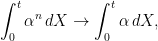
) to  . So, it has a unique continuous linear extensions to the closure of the simple processes. This uniquely defines the integral for progressively measurable integrands such that the right hand side of (4) is finite, as long as it can be shown that they can be approximated by a sequence of simple integrands
  such that
 ![{{\mathbb E}[\int_0^t(\alpha^n-\alpha)^2\,ds]}](https://s0.wp.com/latex.php?latex=%7B%7B%5Cmathbb+E%7D%5B%5Cint_0%5Et%28%5Calpha%5En-%5Calpha%29%5E2%5C%2Cds%5D%7D&bg=ffffff&fg=000000&s=0&c=20201002) tends to zero. In fact, this is achieved by the following approximations
tends to zero. In fact, this is achieved by the following approximations
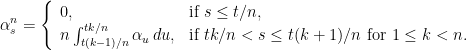 |
(5) |
We still need to extend to the case where  is finite almost surely, rather than requiring it to be integrable. This can be done by applying a localization technique to the Itô isometry: If
  is the first time at which
  , for some constant
  , then the Itô isometry (4) applied to
 ![{1_{(0,\tau]}\alpha}](https://s0.wp.com/latex.php?latex=%7B1_%7B%280%2C%5Ctau%5D%7D%5Calpha%7D&bg=ffffff&fg=000000&s=0&c=20201002) ,
,
Applying the Markov inequality to this gives the following bounds on probabilities.
Combining these gives us the following inequality
which shows that the stochastic integral is continuous in the following sense. If  converges to zero in probability, then convergence of the integrals (3) also holds in probability. Furthermore, if is finite almost surely, then (4) gives such an approximating sequence of simple integrands. Then by uniqueness of continuous extensions of linear maps, it follows that the defining properties given above do indeed uniquely specify the stochastic integral.

tends to zero in probability as
, then
![\displaystyle {\mathbb E}\left[\left(\int_0^{\tau\wedge t}\alpha\,dX\right)^2\right]={\mathbb E}\left[\int_0^{\tau\wedge t}\alpha^2\,ds\right]={\mathbb E}\left[K^2\wedge\int_0^t\alpha^2\,ds\right].](https://s0.wp.com/latex.php?latex=%5Cdisplaystyle++%7B%5Cmathbb+E%7D%5Cleft%5B%5Cleft%28%5Cint_0%5E%7B%5Ctau%5Cwedge+t%7D%5Calpha%5C%2CdX%5Cright%29%5E2%5Cright%5D%3D%7B%5Cmathbb+E%7D%5Cleft%5B%5Cint_0%5E%7B%5Ctau%5Cwedge+t%7D%5Calpha%5E2%5C%2Cds%5Cright%5D%3D%7B%5Cmathbb+E%7D%5Cleft%5BK%5E2%5Cwedge%5Cint_0%5Et%5Calpha%5E2%5C%2Cds%5Cright%5D.+&bg=ffffff&fg=000000&s=0&c=20201002)
![\displaystyle \begin{array}{l} \displaystyle {\mathbb P}\left(\left|\int_0^{\tau\wedge t}\alpha\,dX\right|\ge K\right)\le K^{-2}{\mathbb E}\left[K^2\wedge\int_0^t\alpha^2\,ds\right].\\ \displaystyle {\mathbb P}\left(\tau<t\right)\le K^{-2}{\mathbb E}\left[K^2\wedge\int_0^t\alpha^2\,ds\right]. \end{array}](https://s0.wp.com/latex.php?latex=%5Cdisplaystyle++%5Cbegin%7Barray%7D%7Bl%7D+%5Cdisplaystyle+%7B%5Cmathbb+P%7D%5Cleft%28%5Cleft%7C%5Cint_0%5E%7B%5Ctau%5Cwedge+t%7D%5Calpha%5C%2CdX%5Cright%7C%5Cge+K%5Cright%29%5Cle+K%5E%7B-2%7D%7B%5Cmathbb+E%7D%5Cleft%5BK%5E2%5Cwedge%5Cint_0%5Et%5Calpha%5E2%5C%2Cds%5Cright%5D.%5C%5C+%5Cdisplaystyle+%7B%5Cmathbb+P%7D%5Cleft%28%5Ctau%3Ct%5Cright%29%5Cle+K%5E%7B-2%7D%7B%5Cmathbb+E%7D%5Cleft%5BK%5E2%5Cwedge%5Cint_0%5Et%5Calpha%5E2%5C%2Cds%5Cright%5D.+%5Cend%7Barray%7D+&bg=ffffff&fg=000000&s=0&c=20201002)
![\displaystyle {\mathbb P}\left(\left|\int_0^t\alpha\,dX\right|\ge K\right)\le 2K^{-2}{\mathbb E}\left[K^2\wedge\int_0^t\alpha^2\,ds\right],](https://s0.wp.com/latex.php?latex=%5Cdisplaystyle++%7B%5Cmathbb+P%7D%5Cleft%28%5Cleft%7C%5Cint_0%5Et%5Calpha%5C%2CdX%5Cright%7C%5Cge+K%5Cright%29%5Cle+2K%5E%7B-2%7D%7B%5Cmathbb+E%7D%5Cleft%5BK%5E2%5Cwedge%5Cint_0%5Et%5Calpha%5E2%5C%2Cds%5Cright%5D%2C+&bg=ffffff&fg=000000&s=0&c=20201002)

Hi George, I have a question regarding the final paragraph. How exactly does (4) give an “approximating sequence of simple integrands”?
Also, this definition of the integral for a.s. finite integrands is not done in Karatzas/Shreve and Revuz/Yor. In those books, the integral is defined over [0,\tau^n] , where (\tau^n)_{n \ge 1} is a localising sequence. It’s not so clear to me that the definitions coincide…
Many thanks for your blog.
Hi! You say, “Piecewise constant and left-continuous processes, such as $\alpha$ in (2), which are also adapted are commonly referred to as *simple processes*.” But it seems like $\alpha$ as defined there is right-continuous?
You are right! I fixed it to be consistent.