A Process With Hidden Drift

Consider a stochastic process X of the form

$\displaystyle X_t=W_t+\int_0^t\xi_sds,$

(1)

for a standard Brownian motion W and predictable process ${\xi}$ , defined with respect to a filtered probability space ${(\Omega,\mathcal F,\{\mathcal F_t\}_{t\in{\mathbb R}_+},{\mathbb P})}$ . For this to make sense, we must assume that ${\int_0^t\lvert\xi_s\rvert ds}$ is almost surely finite at all times, and I will suppose that ${\mathcal F_\cdot}$ is the filtration generated by W.

The question is whether the drift ${\xi}$ can be backed out from knowledge of the process X alone. As I will show with an example, this is not possible. In fact, in our example, X will itself be a standard Brownian motion, even though the drift ${\xi}$ is non-trivial (that is, ${\int\xi dt}$ is not almost surely zero). In this case X has exactly the same distribution as W, so cannot be distinguished from the driftless case with ${\xi=0}$ by looking at the distribution of X alone.

On the face of it, this seems rather counter-intuitive. By standard semimartingale decomposition, it is known that we can always decompose

$\displaystyle X=M+A$

(2)

for a unique continuous local martingale M starting from zero, and unique continuous FV process A. By uniqueness, ${M=W}$ and ${A=\int\xi dt}$ . This allows us to back out the drift ${\xi}$ and, in particular, if the drift is non-trivial then X cannot be a martingale. However, in the semimartingale decomposition, it is required that M is a martingale with respect to the original filtration ${\mathcal F_\cdot}$ . If we do not know the filtration ${\mathcal F_\cdot}$ , then it might not be possible to construct decomposition (2) from knowledge of X alone. As mentioned above, we will give an example where X is a standard Brownian motion which, in particular, means that it is a martingale under its natural filtration. By the semimartingale decomposition result, it is not possible for X to be an ${\mathcal F_\cdot}$ -martingale. A consequence of this is that the natural filtration of X must be strictly smaller than the natural filtration of W.

The inspiration for this post was a comment by Gabe posing the following question: If we take ${\mathbb F}$ to be the filtration generated by a standard Brownian motion W in ${(\Omega,\mathcal F,{\mathbb P})}$ , and we define ${\tilde W_t=W_t+\int_0^t\Theta_udu}$ , can we find an ${\mathbb F}$ -adapted ${\Theta}$ such that the filtration generated by ${\tilde W}$ is smaller than ${\mathbb F}$ ? Our example gives an affirmative answer.

Brownian Bridge Construction

The example of a process with hidden drift will be based around the decomposition of a Brownian motion into Brownian bridges or, conversely, the composition of a standard Brownian motion from Brownian bridges. So, I first quickly go over this standard material.

Let us start with a Brownian motion ${X}$ defined over an interval ${[t_0,t_1]}$ . We consider the linear interpolant across the interval,

$\displaystyle \hat X_t=\frac{t_1-t}{t_1-t_0}X_{t_0}+\frac{t-t_0}{t_1-t_0}X_{t_1}$

and the deviation of the process from this interpolation,

$\displaystyle B_t=X_t-\hat X_t.$

It can be seen that B is independent of X at the interval endpoints. It is straightforward to compute the covariances of ${\hat X}$ and ${B_t}$ , which are zero. As the increments of X are jointly normal, independence follows. In fact, B is a Brownian bridge. The process

$\displaystyle W_t=B_t+\int_{t_0}^t\frac{B_s}{t_1-s}ds,$

is a Brownian motion over ${[t_0,t_1]}$ which, again, can be shown by computing covariances. Differentiating, the Brownian bridge B is given from the Brownian motion W via the SDE

$\displaystyle dB_t=dW_t-\frac{B_t}{t_1-t}dt.$

This can be solved to express B in terms of W,

$\displaystyle B_t=(t_1-t)\int_{t_0}^t\frac{dW_s}{t_1-s}$

(3)

Now, suppose we are given the following, for times ${t_0 < t_1}$ , defined on the same probability space.

A random variable ${X_{t_0}}$ .
A standard normal random variable ${U}$ .
A Brownian motion ${W}$ over the interval ${[t_0,t_1]}$ .

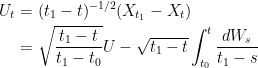
We furthermore suppose that ${X_{t_0}}$ , U and W are independent. The idea is to construct a new Brownian motion X on the interval ${[t_0,t_1]}$ . Taking ${X_{t_0}}$ as specified, we need ${X_{t_1}-X_{t_0}}$ to be normal with variance ${t_1-t_0}$ . This is done by setting

$\displaystyle X_{t_1}=X_{t_0}+(t_1-t_0)^{1/2}U.$

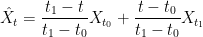
We interpolate X across the interval by inverting the Brownian bridge decomposition above. Constructing a Brownian bridge by (3) and adding this to the linear interpolation of X gives

$\displaystyle \setlength\arraycolsep{2pt} \begin{array}{rl} \displaystyle X_t &\displaystyle = \frac{t_1-t}{t_1-t_0}X_{t_0}+\frac{t-t_0}{t_1-t_0}X_{t_1}+(t_1-t)\int_{t_0}^t\frac{dW_s}{t_1-s}\smallskip\\ &\displaystyle =X_{t_0}+\frac{t-t_0}{\sqrt{t_1-t_0}}U+(t_1-t)\int_{t_0}^t\frac{dW_s}{t_1-s}. \end{array}$

(4)

for all times ${t_0\le t < t_1}$ . This is our desired Brownian motion. Expressing things slightly differently, we have

$\displaystyle dX_t=dW_t+\xi_tdt$

(5)

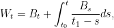
where ${\xi}$ is the process

$\displaystyle \setlength\arraycolsep{2pt} \begin{array}{rl} \displaystyle \xi_t &\displaystyle =\frac{X_{t_1}-X_t}{t_1-t}\smallskip\\ &\displaystyle =\frac{U}{\sqrt{t_1-t_0}}-\int_{t_0}^t\frac{dW_s}{t_1-s}. \end{array}$

(6)

I will also note that, as standard Brownian motion has independent normal increments, for any fixed time ${t\in[t_0,t_1]}$ the random variable

$\displaystyle \setlength\arraycolsep{2pt} \begin{array}{rl} \displaystyle U_t &\displaystyle = (t_1-t)^{-1/2}(X_{t_1}-X_t)\smallskip\\ &\displaystyle =\sqrt{\frac{t_1-t}{t_1-t_0}}U-\sqrt{t_1-t}\int_{t_0}^t\frac{dW_s}{t_1-s} \end{array}$

(7)

will be standard normal and independent of ${X_s}$ over ${s\le t}$ .

Solution to the Hidden Drift Problem

We assume are given a standard Brownian motion W. Start by choosing a strictly increasing sequence of positive times ${\{t_n\}_{n\in{\mathbb Z}}\in{\mathbb R}}$ such that ${t_n\rightarrow\infty}$ as ${n\rightarrow\infty}$ and ${t_n\rightarrow0}$ as ${n\rightarrow-\infty}$ . For example, we can simply take ${t_n=2^n}$ .

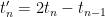Setting ${t_n^\prime=2t_n-t_{n-1}}$ , we have an infinite sequence of overlapping intervals ${[t_{n-1},t^\prime_n]}$ containing ${t_n}$ in their interiors. The idea is to use the Brownian Bridge construction described above to construct X across each of these intervals. To do this, for each n, we need to construct a standard normal random variable ${U_n}$ which is independent of ${\{X_s\colon s\le t_n\}}$ . Given that we have already applied the above construction across the interval ${[t_{n-1},t_n^\prime]}$ , starting with a standard normal ${U_{n-1}}$ , we can construct the new standard normal with the required independence property by (7),

$\displaystyle U_n=\sqrt{\frac{t^\prime_n-t_n}{t^\prime_n-t_{n-1}}}U_{n-1}-\sqrt{t^\prime_n-t_n}\int_{t_{n-1}}^{t_n}\frac{dW_s}{t^\prime_n-s}$

(8)

Since ${(t^\prime_n-t_n)/(t^\prime_n-t_{n-1})=2^{-1}}$ , we can solve this recursive formula as

$\displaystyle U_n=2^{(m-n)/2}U_m-\sum_{k=m+1}^n2^{(k-n)/2}\sqrt{t_k-t_{k-1}}\int_{t_{k-1}}^{t_k}\frac{dW_s}{t^\prime_k-s}$

for any ${m < n}$ . Noting that ${2^{(m-n)/2}\rightarrow0}$ as ${m\rightarrow-\infty}$ , we can take the limit to obtain

$\displaystyle U_n=-\sum_{k=-\infty}^n2^{(k-n)/2}\sqrt{t_k-t_{k-1}}\int_{t_{k-1}}^{t_k}\frac{dW_s}{t^\prime_k-s}.$

(9)

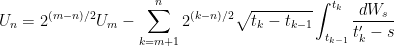
I take (9) as the definition of ${U_n}$ , which we note are a sequence of standard normal random variables satisfying (8), and that ${U_n}$ is ${\mathcal F_{t_n}}$ -measurable. Next, we define X across the interval ${[t_{n-1},t_n]\subseteq[t_{n-1},t^\prime_n]}$ so that it obeys (4) above,

$\displaystyle X_t=X_{t_{n-1}}+\frac{t-t_{n-1}}{\sqrt{t^\prime_n-t_{n-1}}}U_{n-1}+(t^\prime_n-t_{n-1})\int_{t_{n-1}}^t\frac{dW_s}{t^\prime_n-s}.$

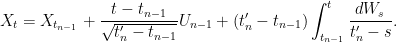
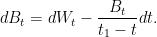
From the construction above, this ensures that ${U_n}$ is independent of the increments of ${X_s}$ over ${s\le t}$ , and that X is a standard Brownian motion. From (5) and (6), we obtain

$\displaystyle X_t=W_t-W_s+X_s+\int_s^t\xi_udu$

(10)

for all times ${0 < s < t}$ , with the drift process

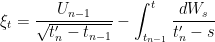$\displaystyle \xi_t =\frac{U_{n-1}}{\sqrt{t^\prime_n-t_{n-1}}}-\int_{t_{n-1}}^t\frac{dW_s}{t^\prime_n-s}$

(11)

over ${t_{n-1}\le t < t_n}$ . In order to take the limit ${s\rightarrow0}$ in (10), we need to show that ${\int\lvert\xi\rvert dt}$ is almost surely finite. From (11), ${\xi_t}$ is standard normal with variance ${(t_n^\prime-t)^{-1}}$ and, hence, ${{\mathbb E}[\lvert\xi_t\rvert]=\sqrt{2/\pi(t^\prime_n-t)}}$ giving,

$\displaystyle \setlength\arraycolsep{2pt} \begin{array}{rl} \displaystyle {\mathbb E}\left[\int_0^{t_n}\lvert\xi_t\rvert dt\right] &\displaystyle =\int_0^{t_n}{\mathbb E}[\lvert\xi_t\rvert]dt =\sqrt{\frac2\pi}\sum_{m=-\infty}^n\int_{t_{m-1}}^{t_m}(t_m^\prime-t)^{-1/2}dt\smallskip\\ &\displaystyle =\sqrt{\frac8\pi}\sum_{m=-\infty}^n\left(\sqrt{t^\prime_m-t_{m-1}}-\sqrt{t^\prime_m-t_m}\right)\smallskip\\ &\displaystyle =(\sqrt2-1)\sqrt{\frac8\pi}\sum_{m=-\infty}^n\sqrt{t_m-t_{m-1}} \end{array}$

So long as ${\sum_{n < 0}\sqrt{t_n-t_{n-1}}}$ is finite, this guarantees that ${\int_0^t\lvert\xi_s\rvert ds}$ is almost surely finite. This is true for the simple case with ${t_n=2^n}$ and, hence, we can take the limit ${s\rightarrow0}$ in (10) to obtain

$\displaystyle X_t=W_t+X_0+\int_0^t\xi_udu.$

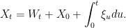
Choose ${X_0=0}$ giving (1) as required.

I finally note that the original motivation for this example was to find a process X satisfying (1) whose natural filtration is strictly smaller than that of W. Letting ${\mathcal G_t}$ be the filtration generated by X, we see that ${U_n}$ is ${\mathcal F_{t_n}}$ -measurable but is independent of ${\mathcal G_{t_n}}$ , directly demonstrating that ${\mathcal G_{t_n}\not\subset\mathcal F_{t_n}}$ .

	Tavin on Class (D) Processes
	George Lowther on Filtrations and Adapted P…
	faceet on Filtrations and Adapted P…
	George Lowther on Filtrations and Adapted P…
	facet on Filtrations and Adapted P…
	Zoltan on Class (D) Processes
	Zoltan on Class (D) Processes
	ARS on Stopping Times and the Debut…
	George Lowther on Upcrossings, Downcrossings, an…
	George Lowther on Stopping Times and the Debut…

A Process With Hidden Drift

Brownian Bridge Construction

Solution to the Hidden Drift Problem

Published by George Lowther

Leave a Reply Cancel reply

Brownian Bridge Construction

Solution to the Hidden Drift Problem

Like this:

Related

Published by George Lowther

Leave a Reply Cancel reply