Brownian Excursions

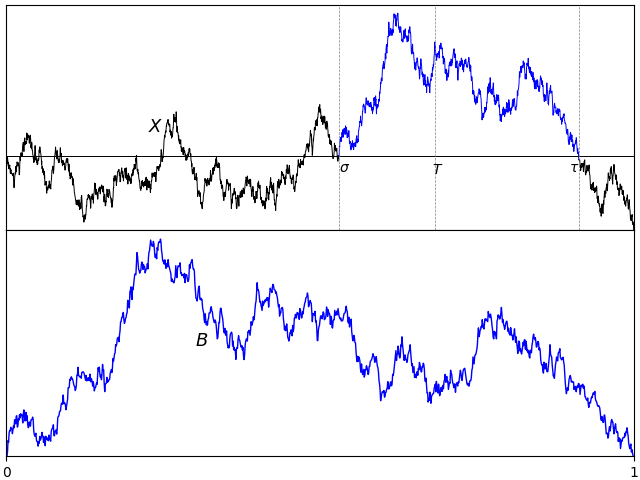
A normalized Brownian excursion is a nonnegative real-valued process with time ranging over the unit interval, and is equal to zero at the start and end time points. It can be constructed from a standard Brownian motion by conditioning on being nonnegative and equal to zero at the end time. We do have to be careful with this definition, since it involves conditioning on a zero probability event. Alternatively, as the name suggests, Brownian excursions can be understood as the excursions of a Brownian motion X away from zero. By continuity, the set of times at which X is nonzero will be open and, hence, can be written as the union of a collection of disjoint (and stochastic) intervals (σ, τ).

In fact, Brownian motion can be reconstructed by simply joining all of its excursions back together. These are independent processes and identically distributed up to scaling. Because of this, understanding the Brownian excursion process can be very useful in the study of Brownian motion. However, there will by infinitely many excursions over finite time periods, so the procedure of joining them together requires some work. This falls under the umbrella of ‘excursion theory’, which is outside the scope of the current post. Here, I will concentrate on the properties of individual excursions.

In order to select a single interval, start by fixing a time T > 0. As X_T is almost surely nonzero, T will be contained inside one such interval (σ, τ). Explicitly,

$\displaystyle \begin{aligned} &\sigma=\sup\left\{t\le T\colon X_t=0\right\},\\ &\tau=\inf\left\{t\ge T\colon X_t=0\right\}, \end{aligned}$

(1)

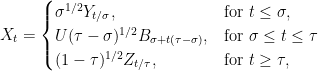
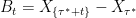
so that σ < T < τ < ∞ almost surely. The path of X across such an interval is t ↦ X_σ + t for time t in the range [0, τ - σ]. As it can be either nonnegative or nonpositive, we restrict to the nonnegative case by taking the absolute value. By invariance, S^-1/2X_tS is also a standard Brownian motion, for each fixed S > 0. Using a stochastic factor S = τ – σ, the width of the excursion is normalised to obtain a continuous process {B_t}_{t ∈ [0, 1]} given by

$\displaystyle B_t=(\tau-\sigma)^{-1/2}\lvert X_{\sigma+t(\tau-\sigma)}\rvert.$

(2)

By construction, this is strictly positive over 0 < t < 1 and equal to zero at the endpoints t ∈ {0, 1}.

Figure 2: Constructing a Brownian excursion

The only remaining ambiguity is in the choice of the fixed time T.

Lemma 1 The distribution of B defined by (2) does not depend on the choice of the time T > 0.

Proof: This follows from scaling invariance of Brownian motion. Consider any other fixed positive time T̃, and use the construction above with T̃, σ̃, τ̃, B̃ in place of T, σ, τ, B respectively. We need to show that B̃ and B have the same distribution. Using the scaling factor S = T̃/T, then X′_t = S^-1/2X_tS is a standard Brownian motion. Also, σ′= σ̃/S and τ′= τ̃/S are random times given in the same way as σ and τ, but with the Brownian motion X′ in place of X in (1). So,

$\displaystyle \tilde B_t=(\tau^\prime-\sigma^\prime)^{-1/2}\lvert X^\prime_{\sigma^\prime+t(\tau^\prime-\sigma^\prime)}\rvert$

has the same distribution as B. ⬜

This leads to the definition used here for Brownian excursions.

Definition 2 A continuous process {B_t}_{t ∈ [0, 1]} is a Brownian excursion if and only it has the same distribution as (2) for a standard Brownian motion X and time T > 0.

In fact, there are various alternative — but equivalent — ways in which Brownian excursions can be defined and constructed.

As a normalized excursion away from zero of a Brownian motion. This is definition 2.
As a normalized excursion away from zero of a Brownian bridge. This is theorem 6.
As a Brownian bridge conditioned on being nonnegative. See theorem 9 below.
As the sample path of a Brownian bridge, translated so that it has minimum value zero at time 0. This is a very interesting and useful method of directly computing excursion sample paths from those of a Brownian bridge. See theorem 12 below, sometimes known as the Vervaat transform.
As a Markov process with specified transition probabilities. See theorem 15 below.
As a transformation of Bessel process paths, see theorem 16 below.
As a Bessel bridge of order 3. This can be represented either as a Bessel process conditioned on hitting zero at time 1., or as the vector norm of a 3-dimensional Brownian bridge. See lemma 17 below.
As a solution to a stochastic differential equation. See theorem 18 below.

An important property of definition (2) is that the normalized excursion is independent of the times σ and τ. Hence, if we wanted to construct a non-normalized excursion on the random interval [σ, τ], we can start with normalized version and, independently, construct the times σ, τ.

Lemma 3 For a standard Brownian motion X and fixed positive time T, the Brownian excursion {B_t}_{t ∈ [0, 1]} defined by (2) is independent of the random times σ, τ.

Proof: Start by choosing a fixed time 0 < S < T and consider the stopping time

$\displaystyle \upsilon=\inf\left\{t\ge S\colon X_t=0\right\}.$

Then, υ ≤ T if and only if σ ≥ S and, by the strong Markov property, X_υ + t is a standard Brownian motion on this event, independent of υ. By scaling invariance,

$\displaystyle Y_t= (1-\upsilon/T)^{-\frac12}X_{\upsilon + t(1-\upsilon/T)}$

is also a standard Brownian motion conditioned on σ ≥ S. Furthermore, the excursion of Y about time T is equal to B so, conditioned on σ ≥ S, B still has the distribution of a Brownian excursion. Hence, B is independent of the event {σ ≥ S} and, therefore, is independent of {σ < S}.

Next, choose times 0 < S < T < U and let

$\displaystyle \tilde\sigma=\sup\left\{t\le U\colon X_t=0\right\}.$

Then, σ̃ < S if and only if X does not hit zero in the interval [S, U], which is equivalent to σ < S and τ > U and, on this event, the excursion B defined about time T coincides with that defined about U. Furthermore, by the argument above, the Brownian excursion defined about the time U is independent of this event, showing that B is independent of the event {σ < S, τ > U}. Finally, all events which are measurable in terms of σ and τ are independent of B, by the pi-system lemma. ⬜

The independence result can be taken further to decompose the Brownian motion into independent components. The term Rademacher distribution describes a random variable which takes the values ±1, each with probability 1/2.

Theorem 4 Let X be a standard Brownian motion, T > 0 be a fixed time and σ < T < τ be as defined by (1). Then, the following collections of random variables are all independent of each other,

the process {B_t}_{t ∈ [0, 1]} defined by (2), which is a Brownian excursion.

the random times {σ, τ}.

sgn(X_T), which has the Rademacher distribution.

the process σ^-1/2X_tσ over 0 ≤ t ≤ 1, which is a standard Brownian bridge.

the process X_τ + t over t ≥ 0, which is a standard Brownian motion.

Proof: By the strong Markov property, X_τ + t is a standard Brownian motion independent of ℱ_τ. Since the other collections are ℱ_τ-measurable, this shows that X_τ + t is independent of all of them.

Next, by lemma 15 of the post on Brownian bridges, Y_t ≡ σ^-1/2X_tσ is a Brownian bridge independent of 1_[σ, ∞)X and, since the other collections are measurable functions of this, Y is independent of all of them.

It only remains to show that the first three collections listed are independent. As the distribution of standard Brownian motion is unchanged under flipping the sign, X → –X, and this transformation does not affect the excursion or the times {σ, τ} but flips the sign of X_T, the sign of X_T must have the Rademacher distribution independently of the first two collections. Finally, we just need to show that the first two collections are independent, but this is stated by lemma 3 above. ⬜

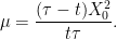
All of the terms in the decomposition of theorem 4 have already-known distributions except for the excursion, which is the subject of this post, and the random times σ, τ. For completeness, we can compute the distribution of these times, which is given by a version of the arcsine law.

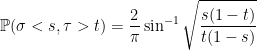
Lemma 5 Let X be a standard Brownian motion, T > 0 be a fixed time and σ < T < τ be as defined by (1). Then,

$\displaystyle {\mathbb P}(\sigma < s, \tau > t) = \frac2\pi\sin^{-1}\sqrt{\frac st}$

for all times 0 ≤ s ≤ T ≤ t.

Proof: The event in question is equivalent to X being nonzero on the interval [s, t] or, equivalently, that the stopping time υ ≡ inf{u ≥ s: X_u = 0} is greater than t. By the strong Markov property, conditioned on υ ≤ t, X_t has a symmetric distribution, so has equal chance of being greater than 0 as being less than 0. So, it has exactly the same probability of being the same sign as X_s as having the opposite sign. This is known as the reflection principle and gives

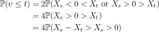$\displaystyle \begin{aligned} {\mathbb P}(\upsilon \le t) &= 2{\mathbb P}(X_s <0<X_t{\rm\ or\ }X_s>0>X_t)\\ &=4{\mathbb P}(X_s > 0 > X_t)\\ &=4{\mathbb P}(X_s-X_t > X_s > 0) \end{aligned}$

Hence, for independent standard normals U, V, we obtain

$\displaystyle \begin{aligned} {\mathbb P}(\upsilon \le t)&=4{\mathbb P}(\sqrt{t-s}U > \sqrt{s}V > 0)\\ &= 4{\mathbb P}(U\cos\theta > V\sin\theta > 0) \end{aligned}$

where θ is the angle between 0 and π/2 such that sinθ = √s/t and cosθ = √1 - s/t. By symmetry, the angle between the x-axis and (U, V) is uniformly distributed over [0, 2π], and the condition that Ucosθ > Vsinθ > 0 says that it lies between 0 and π/2 – θ. Hence,

$\displaystyle {\mathbb P}(\upsilon \le t)=\frac2\pi(\pi/2-\theta)$

giving

$\displaystyle {\mathbb P}(\sigma < s, \tau > t) ={\mathbb P}(\upsilon > t)=\frac2\pi\theta$

as required. ⬜

The fact that the excursion B is independent of (σ, τ) and of the Brownian motion outside of this interval means that if we construct the excursions about a set of distinct times then, conditional on their intervals being disjoint, the excursions are independent. This is the situation in figure 1 above where several excursions are plotted for the same Brownian motion path. We could take this idea to its logical conclusion and consider the set of all excursions of a Brownian motion sample path. These will be independent of each other and of the zero-set of the original path, so the Brownian motion can be reconstructed by ‘filling in the gaps’ of the set of times where it is zero. This is best understood as part of excursion theory, so I will not go deeply into it here.

Since the original Brownian motion sample path can be reconstructed from the collections listed, theorem 4 provides a useful alternative construction of the Brownian motion from several independent components.

Brownian bridge excursions

Rather than starting with Brownian motion, we can equally well construct excursions from the sample paths of a Brownian bridge. This works in exactly the same way — compare figures 2 and 3.

Theorem 4 also follows across to this case in a straightforward fashion.

Theorem 6 Let 0 < T < 1 be a fixed time, X be a standard Brownian bridge, and σ < T < τ be as defined by (1). Then the process {B_t}_{t ∈ [0, 1]} defined by (2),

$\displaystyle B_t=(\tau-\sigma)^{-1/2}\lvert X_{\sigma+t(\tau-\sigma)}\rvert$

is a Brownian excursion. More precisely, the following collections of random variables are all independent of each other,

the Brownian excursion B defined by (2).

the random times {σ, τ}.

sgn(X_T), which has the Rademacher distribution.

the process σ^-1/2X_tσ over 0 ≤ t ≤ 1, which is a standard Brownian bridge.

the process (1 - τ)^-1/2X_{τ + t(1 - τ)} over 0 ≤ t ≤ 1, which is a standard Brownian bridge.

Proof: Let us start with the case where X is a Brownian motion, so that theorem 4 can be applied. Then, the first 4 collections of random variables in the statement of the theorem are independent with stated distributions and, independently, Y_t = X_τ + t is a standard Brownian motion.

Defining the random time υ = sup{t ≤ 1: X_t = 0}, lemma 15 of the post on Brownian bridges says that X̃_t = υ^-1/2X_tυ is a Brownian bridge independent of υ.

Restricting to the event υ > T, we have σ < τ < υ. Writing T̃ = T/υ then σ̃ = σ/υ is the last time before T̃ at which X̃_σ̃ = 0 and τ̃ = τ/υ is the first time after T̃ for which X̃_τ̃ = 0. So, the following collections of random variables are independent:

B_t = (τ - σ)^-1/2|X_{σ + t(τ - σ)}|= (τ̃ - σ̃)^-1/2|X̃_{σ̃ + t(τ̃ - σ̃)}|, which is a Brownian excursion.
The random times {σ̃, τ̃}.
sgn(X_T) = sgn(X̃_T̃), which has the Rademacher distribution.
The process σ^-1/2X_tσ = σ̃^-1/2X_tσ̃ over 0 ≤ t ≤ 1, which is a Brownian bridge.
The process Ỹ_t = (1 - τ)^-1/2Y_{t(1 - τ)} which is a standard Brownian motion (by the scaling property).

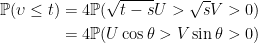
The process in the last bullet point of the statement of the theorem (defined in terms of the Brownian bridge X̃) can be expressed as

$\displaystyle \begin{aligned} (1-\tilde\tau)^{-1/2}\tilde X_{\tilde\tau+t(1-\tilde\tau)} &=(\upsilon-\tau)^{-1/2}X_{\tau+t(\upsilon-\tau)}\\ &=(\upsilon-\tau)^{-1/2}Y_{t(\upsilon-\tau)}\\ &=\rho^{-1/2}\tilde Y_{t\rho} \end{aligned}$

where ρ = (υ - τ)/(1 - τ) is the final time before 1 for which Ỹ_ρ = 0. Lemma 15 of the post on Brownian bridges says that this is a Brownian bridge.

We have proven the result in terms of the Brownian bridge X̃ and with the fixed time T replaced by T̃ = T/υ, where υ is a random variable taking values in ${(T,1)}$ independently of X̃. Conditioning on υ > 1 – ϵ for arbitrarily small ϵ > 0 gives the result. ⬜

The arcsine law for the distribution of the times σ, τ stated in lemma 5 carries across to the construction from Brownian bridges.

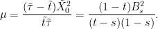
Lemma 7 Let X be a standard Brownian bridge, 0 < T < 1 be a fixed time and σ < T < τ be as defined by (1). Then,

$\displaystyle {\mathbb P}(\sigma < s, \tau > t) = \frac2\pi\sin^{-1}\sqrt{\frac{s(1-t)}{t(1-s)}}$

for all times 0 ≤ s ≤ T ≤ t ≤ 1.

Proof: Using the fact that Y_t = (1 + t)X_{t/(1 + t)} is a Brownian motion, vanishing at times t̃ = t/(1 - t) whenever X vanishes at t, lemma 5 gives

$\displaystyle \begin{aligned} {\mathbb P}(\sigma < s, \tau > t) &={\mathbb P}(\tilde\sigma < \tilde s, \tilde\tau >\tilde t)\\ &= \frac2\pi\sin^{-1}\sqrt{\frac{\tilde s}{\tilde t}} \end{aligned}$

as required. ⬜

In passing, I note that the fact we can construct excursions from Brownian bridges, whose law is symmetric under time reversal means that the Brownian excursion distribution is also symmetric under time reversal.

Lemma 8 If B_t is a Brownian excursion then so is B_1 - t.

Proof: By theorem 6, we can suppose that B is the normalized excursion of a Brownian bridge X about a time 0 < T < 1. Then, B_1 - t is the normalized excursion of X_1 - t about the time 1 – T, so is also a Brownian excursion. ⬜

As promised above, we can show that excursions can be expressed as Brownian bridges conditioned on being positive but, as this requires conditioning on a zero probability event, we need to be careful. We approximate by conditioning on B being close to a positive process and show that this converges in the limit. There are various different ways in which this approximation can be done. Here, I consider conditioning on the process being positive for all t in the unit interval except near the end-points. This turns out to be relatively straightforward, although other methods also work (such as conditioning on the minimum of the process being not too small, or on the process being nonnegative at finite sets of times).

By definition, the distribution of a process X under probability measures ℙ_n converges weakly to its law under ℙ if 𝔼_{ℙ_n}[f(X)] → 𝔼_ℙ[f(X)] for any bounded continuous function f of the paths of X. The topology of uniform convergence is used.

Theorem 9 Let {X_t}_{t ∈ [0, 1]} be a Brownian bridge, and 0 < a_n < b_n < 1 be reals with a_n → 0 and b_n → 1. Then, the distribution of X conditioned on inf_{t ∈ [a_n, b_n]}X_t > 0 converges weakly to that of a Brownian excursion as n → ∞.

Proof: Fixing a time 0 < T < 1, theorem 6 says that we can write

$\displaystyle X_t=\begin{cases} \sigma^{1/2}Y_{t/\sigma},&{\rm for\ }t\le\sigma,\\ U(\tau-\sigma)^{1/2}B_{\sigma+t(\tau-\sigma)},&{\rm for\ }\sigma\le t\le\tau\\ (1-\tau)^{1/2}Z_{t/\tau},&{\rm for\ }t\ge\tau,\\ \end{cases}$

for Brownian bridges Y,Z, random times {σ, τ}, Rademacher variable U and Brownian excursion U. In particular, X converges uniformly to B as σ → 0 and τ → 1. Furthermore, each of these terms is independent.

So long as T is in the interval (a_n, b_n) then the event

$\displaystyle S_n=\left\{\inf_{t\in[a_n,b_n]}X_t > 0\right\}$

is equivalent to σ < a_n, τ > b_n and U = 1. So, conditioned on S_n, as n goes to infinity, the distribution of X converges weakly to that of B which, by independence with S_n, is a Brownian excursion. ⬜

The Vervaat transformation

I now describe an interesting link between Brownian bridges and excursions. There is a straightforward conversion from Brownian bridges to excursions on a path-by-path basis.

If X is a Brownian bridge, let τ^∗ be the time at which it attains its minimum so that X_t ≥ X_τ^∗ for all times t in the unit interval. This minimum is achieved at a unique time, almost surely. We switch around the paths of X on the intervals [0, τ^∗] and [τ^∗, 1], and subtract the minimum value X_τ^∗. The resulting sample path B has the Brownian excursion distribution. That is, B_t is equal to X_{τ^∗ + t} – X_τ^∗ when t ≤ 1 – τ^∗ and X_{τ^∗ + t - 1} – X_τ^∗ when t ≥ 1 – τ^∗. Equivalently, B_t = X_s – X_τ^∗ where s = τ^∗ + t modulo 1.

Going in the opposite direction, starting with an excursion B, choose a time υ uniformly distributed on the unit interval independent from B. Switching around the paths of B on the intervals [0, υ] and [υ, 1], and subtracting B_υ, gives a Brownian bridge.

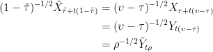
This mapping between bridges and excursions is demonstrated in figure 4 below. The top plot is of a Brownian bridge sample path. The path before the minimum is attained is shown in blue, and the part after is in green. Switching the order of these segments and shifting vertically to make it start from zero gives the Brownian excursion path in the bottom plot.

This map from Brownian bridge paths to excursions was discovered by Vervaat, and is known as the Vervaat transform.

Brownian bridge to excursion — Figure 4: Transforming a Brownian bridge into a Brownian excursion

As was noted in the posts on Brownian bridges and their Fourier expansions, for a continuous process X_t with time index t ranging over the unit interval, it can be useful to extend the time index to the entire real line. This is done by making it periodic so that X_t + n = X_t for integer n. The periodic extension can be written as X_{t} where {t} is the fractional part of t. So long as X₀ = X₁, the extension will be continuous.

With this notation, the Vervaat transform says that if X is a Brownian bridge then X_{{τ^∗ + t}} – X_τ^∗ is an excursion. That is, if we translate the time index of the bridge so that its minimum is at time 0, and translate its value so that it starts at 0, then we get a Brownian excursion. Immediate consequences of this result include the fact that the range max_tX_t – min_tX_t of a Brownian bridge X has the same distribution as the maximum of a Brownian excursion. It is interesting to that when these distributions were calculated in 1976 by Chung (Excursions in Brownian motion) and Kennedy (The Distribution of the Maximum Brownian Excursion), the fact that they are the same was seen as a curiosity.Vervaat only published his paper in 1979 providing the probabilistic reason for this apparent coincidence.

I start by proving a discrete-time version of the transform, which is much more straightforward.

Lemma 10 Let {X_t}_{t ∈ [0, 1]} be a Brownian bridge and n be a positive integer. Then, X_t almost surely has a unique minimum for t in the set {k/n: k = 0, 1, …, n – 1}. If we let τ_n be the time this minimum it attained, then the process X_{{τ_n + t}} – X_{τ_n} has the same distribution as X has when conditioned on the event

$\displaystyle S_n=\left\{\min_{k=1,2,\ldots,n-1}X_{\frac kn} > 0\}\right\}.$

Proof: From the Brownian bridge covariance structure, for times 0 ≤ s < t < 1, X_t – X_s is normal with nonzero variance, so is almost surely not equal to 0. Hence, for time restricted to a finite subset of [0, 1), the values of X_t are all distinct and so it has a unique minimum.

Now choose a random variable υ uniformly distributed on {0/n, 1/n, …, (n - 1)/n} independently of X. As previously shown, the process Y_t = X_{υ + t} – X_υ is also a Brownian bridge so has the same distribution as X. Conditioning on υ = τ_n does not affect the distribution of X, and gives Y_t = X_{{τ_n + t}} – X_{τ_n}.

On the other hand, υ = τ_n if and only if Y_t > 0 for t in {1/n, 2/n, …, , (n - 1)/n}, so conditioning on this event gives the same distribution for Y as X has conditioned on S_n. ⬜

The idea is that, by letting n go to infinity, the law of X conditioned on X_k/n > 0 over 0 < k < n tends to a Brownian excursion and that τ_n tends to τ^∗. Taking this limits will give the result. First, though, we need to show that continuous-time Brownian bridges have a unique minimum.

Lemma 11 If X is a Brownian bridge then, with probability one, there is a unique time 0 ≤ τ^∗ < 1 at which X_τ^∗ = min_tX_t.

Proof: We can reduce to the case where X is standard Brownian motion. Letting σ = sup_t ≤ 1X_t, then lemma 15 of the post on Brownian bridges says that B_t = σ^-1/2X_tσ is a Brownian bridge independently of 1_[σ, 1]X. If B did not have a unique minimum, then the same would be true of X whenever X₁ > 0, which has probability 1/2. So, it is sufficient to show that Brownian motion X has a unique minimum.

If X did not have a unique minimum, then for some rational time 0 < t < 1 we would have min_s ≤ tX_s = min_s ≥ tX_s with positive probability. That is, the independent Brownian motions X_t – X_t - s and X_t – X_t + s (with time index s ≥ 0) would have the same maximum. However, the maxima are independent with a continuous distribution, so are almost surely distinct. ⬜

Theorem 12 (Vervaat) Let {X_t}_{t ∈ [0, 1]} be a Brownian bridge and τ^∗ ∈ [0, 1) be the time at which its minimum is achieved, Then, τ^∗ is uniformly distributed and, independently,

$\displaystyle B_t=X_{\{\tau^*+t\}}-X_{\tau^*}$

is a Brownian excursion over 0 ≤ t ≤ 1.

Proof: Use the notation of lemma 10. As X has a unique minimum and is continuous, then τ_n → τ As n goes to infinity. So, the processes Bⁿ_t ≡ X_{{τ_n + t}} – X_{τ_n} converge uniformly to B_t.

On the other hand, the law of Bⁿ_t is the same as X_t conditioned on S_n. Fixing a time 0 < T < 1, by theorem 4 we can write

$\displaystyle X_t=U(\tau-\sigma)^{-1/2}Y_{(t-\sigma)/(\tau-\sigma)}$

over σ ≤ t ≤ τ, for random times σ < T < τ, a Rademacher random variable U and, independently, a Brownian excursion Y. As the events S_n only depend on the signs of X, it does not depend on Y, so is independent of Y. Therefore, conditioned on S_n, Y is still a Brownian excursion.

Next, for any 0 < a < T < b < 1 then, as Bⁿ tends uniformly to B, for large enough n it will be strictly positive on the interval [a, b]. So,

$\displaystyle \begin{aligned} {\mathbb P}(\sigma < a, \tau > b, U=1\vert\; S_n) &={\mathbb P}\left(\min_{t\in[a,b]}X_t > 0\Big\vert\; S_n\right)\\ &={\mathbb P}\left(\min_{t\in[a,b]}B^n_t > 0\right)\\ &\rightarrow1 \end{aligned}$

as ${n\rightarrow\infty}$ . So, conditioned on S_n, σ → 0, τ → 1, U → 1 in law. Hence, X tends in law to the Brownian excursion Y. As it also tends to B, this shows that B is a Brownian excursion.

It only remains to show that τ^∗ is uniformly distributed independently of B. To this end, introduce a random variable υ uniformly distributed on [0, 1) independently of X, and set X̃_t = X_{υ + t} – X_υ, which is a Brownian bridge. Its minimum occurs at time τ̃^∗ = {τ^∗ – υ} and X̃_{{τ̃^∗ + t}} – X̃_τ̃^∗ = B_t. Hence, τ̃^∗ is uniformly distributed independently of B but, by construction, (B, τ̃^∗) has the same distribution as (B, τ^∗). ⬜

We can also go in the opposite direction and construct Brownian bridges from the sample paths of excursions.

Theorem 13 Let {B_t}_{t ∈ [0, 1]} be a Brownian excursion and, independently, υ be uniformly distributed on [0, 1). Then, X_t = B_{υ + t} – B_τ is a standard Brownian bridge.

Proof: Start by choosing X to be a Brownian bridge. By theorem 12 it has a unique minimum at time τ^∗ ∈ [0, 1), which is uniformly distributed and independent of the excursion B_t = X_{{τ^∗ + t}} – X_τ^∗.

Rearranging, X_t = B_{υ + t} – B_υ is a standard Brownian bridge where υ = 1 – τ^∗ is uniformly distributed on (0, 1) independently of B. ⬜

The excursion distribution

We can show that Brownian excursions are Markov processes and compute their transition probabilities. It turns out these are described by noncentral chi-squared distributions. Recall that χ²_n(μ) is the distribution of the sum of squares of independent normally distributed random variables,

$\displaystyle Z_1^2+Z_2^2+\cdots+Z_n^2,$

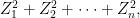where Z_i have unit variances and means μ_i satisfying Σ_iμ_i² = μ. Alternatively, the distribution of a χ²_n(μ) random variable Z is described by the moment generating function,

$\displaystyle {\mathbb E}[e^{-\lambda Z}]=(1+2\lambda)^{-\frac n2}\exp\left(\frac{-\lambda\mu}{1+2\lambda}\right)$

for λ ≥ 0. This also serves as a valid definition for noninteger n, although that will not be required here. In fact, we only require chi-squared distributions for order n = 3. Start by looking at the distribution of a Brownian motion conditioned on when it hits zero.

Lemma 14 Let X be Brownian motion with initial value X₀ > 0 and

$\displaystyle \tau=\inf\{t\ge0\colon X_t=0\}$

be the first time that it hits 0. Then, for any time t > 0, conditioned on the values of X₀ and τ > t,

$\displaystyle \frac{\tau X^2_{t}}{t(\tau-t)}$

has the χ²₃(μ) distribution where

$\displaystyle \mu=\frac{(\tau-t)X_0^2}{t\tau}.$

Proof: Throughout, I will condition on the value of X₀ > 0, so this can be taken to be constant. Fixing a time T > t, we start by computing the distribution of X_t on the event τ > T using the expression

$\displaystyle {\mathbb E}[f(X_t^2)1_{\{\tau > T\}}]={\mathbb E}[f(X_t^2){\rm sgn}(X_T)].$

This is the reflection principle. By symmetry in reflecting X about 0 after time τ, the expectation on the right hand side restricted to τ ≤ T is zero and, restricted to τ > T, it is equal to the left hand side.

As X_T – X_t is a centered normal with variance T – t independently of X_t, we obtain

$\displaystyle {\mathbb E}[f(X_t^2)1_{\{\tau > T\}}]={\mathbb E}[f(X_t^2)(2\Phi(X_t/\sqrt{T-t})-1)]$

where Φ is the cumulative normal distribution function Φ(x) = ℙ(N < x) for standard normal N. As this has derivative e^–x²/2/√2π, the expression above is continuously differentiable in T, so regular continuous conditional probabilities exist with respect to τ. Taking the derivative,

$\displaystyle {\mathbb E}[f(X_t^2)\vert\;\tau=T]\sim{\mathbb E}[f(X_t^2)e^{-\frac12X_t^2/(T-t)}X_t].$

I am using ∼ to mean that the two sides are equal up to a nonzero scaling factor depending only on t, T, X₀. This avoids a bit of mess since we do not need to keep of these scaling factors which, in any case, are uniquely determined by the fact that the total probability must sum to one.

We compute the moment generating function of Y = τX_t²/(t(τ - t)) by setting f(x) = e^{–λTx/(t(T - t))},

$\displaystyle {\mathbb E}[e^{-\lambda Y}\vert\;\tau=T]\sim{\mathbb E}[e^{-\frac{a}{2}X_t^2}X_t]$

where a = 2λT/(t(T - t)) + 1/(T - t). We are effectively done now. We know that X_t is normal with mean X₀ and variance t, so have everything necessary to compute the expectation on the right hand side. We could just plug in the probability density of X_t and perform the integral. To avoid some of the messy details, we can use some of the ideas from the post on the normal distribution. By equation (12) from that post,

$\displaystyle {\mathbb E}[e^{-\frac{a}{2}X_t^2}]=(1+at)^{-1/2}e^{-\frac{a X_0^2}{2(1+at)}}$

As X_t has mean X₀, we can differentiate wrt this, so that X_t has derivative equal to 1 giving,

$\displaystyle \begin{aligned} {\mathbb E}[e^{-\frac{a}{2}X_t^2}X_t]&=X_0(1+at)^{-3/2}e^{-\frac{a X_0^2}{2(1+at)}}\\ &= X_0(1+at)^{-3/2}e^{-\frac{\lambda\mu}{1+2\lambda}-\frac{X_0^2}{2T}}\\ &\sim (1+2\lambda)^{-3/2}e^{-\frac{\lambda\mu}{1+2\lambda}} \end{aligned}$

with μ = (T - t)X₀²/(tT), where I used 1 + at ∼ 1 + 2λ. As this is the moment generating function of the χ²₃(μ) distribution, the proof is complete. ⬜

Applying the result above to Brownian excursions gives the transition probabilities.

Theorem 15 A continuous nonnegative process {B_t}_{t ∈ [0, 1]} with natural filtration ℱ_· is a Brownian excursion if and only if B₀ = 0 and, for times 0 ≤ s < t < 1 then, conditioned on ℱ_s,

$\displaystyle \frac{(1-s)B^2_t}{(1-t)(t-s)}$

has the χ²₃(μ) distribution where

$\displaystyle \mu= \frac{(1-t)B^2_s}{(1-s)(t-s)}.$

Proof: We just need to prove that an excursion B has these conditional distributions since, in the opposite direction, Markov processes are uniquely determined by their initial condition and transition function.

It is sufficient to consider times 0 < s < t < 1, since the case with s = 0 following by taking the limit as s tends to 0. Using theorem 4, we can consider a Brownian excursion given by (2),

$\displaystyle B_u = (\tau-\sigma)^{-1/2}\lvert X_{\sigma+u(\tau-\sigma)}\rvert$

for standard Brownian motion X, with σ being the final time before 1 at which X_σ = 0 and τ being the first time after 1 for which X_τ = 1. We condition on σ = 1 – s and τ = 1 + σ, which are independent of B, and on the values of X_u over u ≤ 1. Then, X̃_u = X_1 + u is a Brownian motion conditioned on hitting 0 at time τ̃ = 1 – s and B_t = X̃_t̃ where t̃ = t – s. Then,

$\displaystyle \frac{(1-s)B_t^2}{(1-t)(t-s)}=\frac{\tilde\tau\tilde X_{\tilde t}^2}{\tilde t(\tilde\tau - \tilde t)}$

which, by lemma 14, has the χ²₃(μ) distribution with

$\displaystyle \mu=\frac{(\tilde\tau-\tilde t)\tilde X_0^2}{\tilde t\tilde\tau}=\frac{(1-t)B_s^2}{(t-s)(1-s)}.$

⬜

There is already a standard class of Markov processes described by noncentral chi-squared distributions. Specifically, Bessel processes. A nonnegative continuous Markov process X is a BES²_n process if for all times s < t then, conditioned on X_s, X_t/(t - s) has the χ²_n(X_s/(t - s)) distribution. This is referred to as a squared Bessel process. A (non-squared) Bessel process is the square root of a BES²_n process, which I denote by BES_n. Then, squared and non-squared Bessel processes with initial value a will be denoted by BES²_n(a) and BES_n(a) respectively. A word of warning on the notation: where I use BES_n(a), some authors use BES_a(n). There does not seem to be a universally agreed standard here so, when comparing results in these notes with other sources, the meaning of the notation should be checked.

Brownian excursion sample paths can be constructed as a simple transform of the paths of a Bessel process of order 3.

Theorem 16 A continuous process {B_t}_{t ∈ [0, 1]} is a Brownian excursion if and only if (1 + t)B_{t/(1 + t)} is a BES₃(0) process. Equivalently, B_t = (1 - t)X_{t/(1 - t)} for a BES₃(0) process Y.

Proof: The two conditions are clearly equivalent, since (1 + t)B_{t/(1 + t)} = X_t if and only if B_t = (1 - t)X_{t/(1 - t)}. Supposing that X is a BES₃(0), it needs to be shown that B is a Brownian excursion.

Let ℱ_· and 𝒢_· be the natural filtrations of B and X respectively, so that ℱ_t = 𝒢_{t/(1 - t)}.

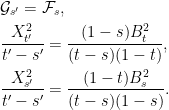For times 0 ≤ s < t < 1, set s′= s/(1 - s) and t′= t/(1 - t). By definition, conditional on ${\mathcal G_{s'}}$ , X²_t′/(t′-s′) has the χ²₃(μ) distribution with μ = X²_s′/(t′-s′). A little rearrangement gives

$\displaystyle \begin{aligned} &\mathcal G_{s'}=\mathcal F_s,\\ &\frac{X^2_{t'}}{t'-s'}=\frac{(1-s)B^2_t}{(t-s)(1-t)},\\ &\frac{X^2_{s'}}{t'-s'}=\frac{(1-t)B^2_s}{(t-s)(1-s)}. \end{aligned}$

From theorem 15, B is a Brownian excursion. ⬜

Brownian excursions can be identified as Bessel bridges, which are Bessel processes started from zero and conditioned on hitting zero at time 1. Alternatively, they can be constructed as the vector norm

$\displaystyle \lVert X_t\rVert = \sqrt{(X^1_t)^2+(X^2_t)^2+\ldots+(X^n_t)^2}$

of an n-dimensional Brownian bridge X. That is, X = (X¹, X², …, Xⁿ) for independent Brownian bridges X¹, …, Xⁿ. To see this, consider an n-dimensional Brownian motion X, so its vector norm B = ‖X‖ is a ${{\rm BES}_n(0)}$ process. Conditioning on B₁ being small is equivalent to conditioning on each individual Xⁱ₁ being small so, in the limit, expresses B conditioned on B₁ = 0 as the vector norm of an n-dimensional Brownian bridge.

Theorem 17 A Bessel bridge of order 3 is a Brownian excursion. That is, if X = (X¹, X², X³) is a 3-dimensional Brownian bridge, then ‖X‖ is a Brownian excursion.

Proof: As Xⁱ are independent Brownian bridges, t ↦ (1 + t)Xⁱ_{t/(1 + t)} are independent Brownian motions and, hence, (1 + t)‖X_{t/(1 + t)}‖ is a BES₃(0) process. Then theorem 16 says that ‖X‖ is a Brownian excursion. ⬜

The excursion SDE

The final method I use to represent Brownian excursions is via a stochastic differential equation (SDE). Recall the Brownian bridge SDE which included the negative drift term –B_t/(1 - t) pushing it to zero at time 1. We expect the SDE for a Brownian excursion B to have a similar drift term but, as it is nonnegative, there should also be a positive drift term which goes to infinity as B goes to zero to push it away. In fact, we show that it satisfies the SDE

$\displaystyle dB_t=dW_t+\left(\frac1{B_t}-\frac{B_t}{1-t}\right)dt.$

(3)

Theorem 18 A nonnegative continuous process ${\{B_t\}_{t\in[0,1]}}$ is a Brownian excursion if and only if ${B_0=0}$ (almost surely) and it solves the SDE (3) over 0 < t < 1 for a standard Brownian motion ${\{W_t\}_{t\in[0,1]}}$ .

Proof: We are spoilt for choice on how to solve this. We could use the transition probabilities directly (as was done for Brownian bridges), or use the identification with Bessel bridges. Instead, I will use representation in terms of Bessel processes. Recall the SDE for a BES²_n process Y

$\displaystyle dY = 2\sqrt{Y}dW+ndt$

for Brownian motion W. Then, for a non-squared Bessel process Y we write X = Y², and by an application of Ito’s lemma with n = 3,

$\displaystyle dX = dW+X^{-1}dt.$

(4)

Consider the time-changed process B_t = (1 - t)X_{t/(1 - t)}. Note that W_{t/(1 - t)} is centered Gaussian with independent increments and variance t/(1 - t). As this has derivative (1 - t)^-2 we can write dW_{t/(1 - t)} = (1 - t)^-1dW̃_t for a standard Brownian motion W̃. Then, SDE (4) is equivalent to B satisfying

$\displaystyle \begin{aligned} dB_t &= (1-t)dX_{t/(1-t)}-X_{t/(1-t)}dt\\ &=d\tilde W_t+B_t^{-1}dt-(1-t)^{-1}B_tdt, \end{aligned}$

which is SDE (3) with respect to a different Brownian motion. Hence, B satisfies (3) if and only if X satisfies (4) for some other Brownian motion or, equivalently, X is a BES₃ process. So, the result follows from theorem 16. ⬜

	Tavin on Class (D) Processes
	George Lowther on Filtrations and Adapted P…
	faceet on Filtrations and Adapted P…
	George Lowther on Filtrations and Adapted P…
	facet on Filtrations and Adapted P…
	Zoltan on Class (D) Processes
	Zoltan on Class (D) Processes
	ARS on Stopping Times and the Debut…
	George Lowther on Upcrossings, Downcrossings, an…
	George Lowther on Stopping Times and the Debut…