Martingale Marginals

[This post originates from twitter threads posted on 9 Sep 21 and 2 Feb 22.]

A while ago, I proved the result: A continuous strong Markov martingale is uniquely determined by its marginal distributions. This is discussed in a recent paper by Beiglböck, Pammer, and Schachermayer.

Time for a thread discussing some of these ideas, which have been studied for decades in both stochastic calculus and mathematical finance.

➢ This is a surprisingly subtle result, which is difficult to prove in full generality. I managed this in the following paper, but the proof is long.

➢ I will go over some of the history of this problem, before moving on to my own contributions. First, let’s start with the basics:

• A (real valued) martingale X_t is a random process where at any time t, its future expected values (conditional on all currently observable information) equals the current value:
  

  for times t ≤ T. E.g., standard Brownian motion, the cumulative winnings playing a fair gambling game, etc.

• Next, the (1-dimensional) marginals are the distributions of X_t at each individual time t. This is way too little information to infer the joint distributions. But, what about if X is known to be a martingale?

➢ The question has a long history. Lévy proved various characterisations for a continuous martingale to be a Brownian motion. E.g., if X_t² – t is also a martingale, or if X has IID increments.

➢ In 1972 Kellerer proved a necessary and sufficient condition for a martingale to exist matching a given set of marginals: They must be increasing in the convex order. This means that E[f(X_t)] must be increasing in t, for all convex functions f.

A stochastic process or collection of marginal distributions which is increasing in the convex order is sometimes referred to as a ‘peacock’, which is a pun on the French acronym PCOC for “processus croissant pour l’ordre convex”.

➢ The necessity of Kellerer’s condition follows easily from Jensen’s inequality. The significance of the result is that it is also sufficient for such a martingale to exist.

But is it uniquely determined by the marginals? Financial option pricing theory has a lot to say.

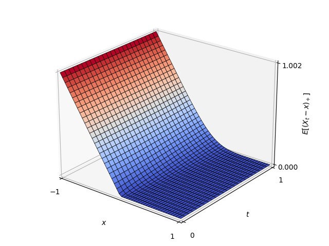
➢ The prices of a traded financial asset through time can be modelled as a martingale X_t. Then, the time-0 price of a call option on that asset of strike price x and maturity t is:

This is fully determined by the marginals of X and, in the other direction, the distribution function of X_t is obtained as the derivative C_x(t, x).

➢ So, having call prices C(t, x) of all strikes and maturities is the same as having the marginals. As call options are traded in the markets, their prices are often known.

C(t, x) is automatically convex in x, and the property of being increasing in t is equivalent to the marginals increasing in the convex order.

➢ Local volatility is a popular option pricing model. This specifies the asset price X as a solution to the stochastic differential equation (SDE)

for driving Brownian motion B and local volatility surface σ. In 1994 Bruno Dupire noted that option prices satisfy the partial differential equation (PDE)

As the probability density of X_t is given by the second derivative C_xx(t, x), Dupire’s approach links the call prices/marginal densities to the local volatility. This requires that the call prices are smooth and C_xx is strictly positive.

➢ So, given marginal distributions, the local volatility method is to back out the local vol surface σ,

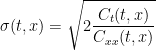and solve the SDE

to find a martingale X with the required marginals.

➢ So, there is a unique local volatility model matching given marginals! At least, subject to various smoothness and regularity constraints on the option prices and volatilities…

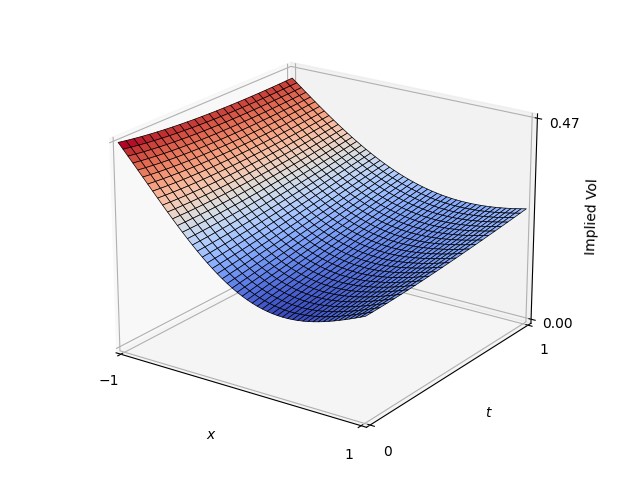
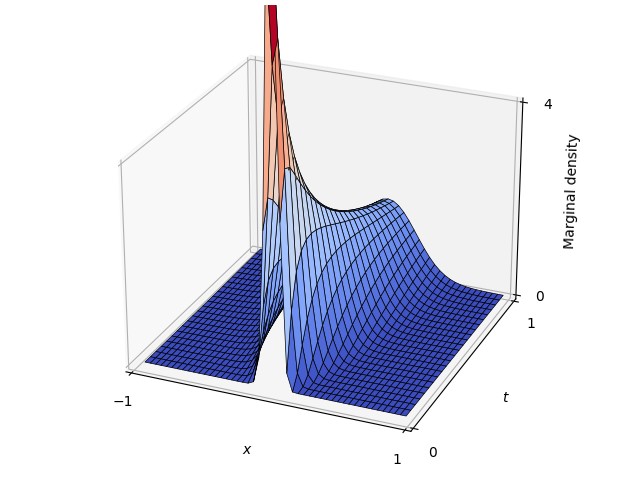
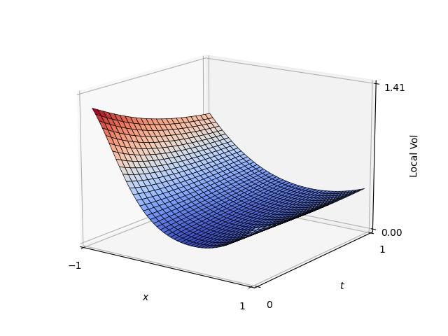
➢ The images below show an example where the marginals are chosen according to the plotted ‘implied volatilities’. The (normal) implied volatility for each maturity time t and strike price x is, by definition, the constant value of volatility at which the call price equals C(t, x). That is, E[(X_t - x)⁺] is equal to same value as if X_t is normal with mean 0 and standard deviation σ_imp(t, x)√t. Implied volatilities are just a convenient alternative way of quoting call prices. I also show the call prices, the marginal densities, and the obtained local vols.

---

Moving on to my own contributions to this problem, we start with the question: what can we do if the call prices C(t, x) are not smooth? We could try approximating by smooth functions but, in the limit, the local volatilities will not converge to anything, and will oscillate wildy.

➢ We can hope for the following: when the local vols are plugged into the SDE and we compute the joint distributions of the martingale X, the oscillations all cancel out when we take the limit. There does not seem to be any way to take this limit directly using the SDE…

➢ …but there is one property which suggests that the limit does have well-defined distributions. As we are fitting specified marginals we know, by construction, that these one-dimensional marginals will converge. Is it such a stretch to suppose that the joint distributions also converge to a limit?

➢ Rather than using the SDE above, the local vol model can be described by a ‘backwards equation’. For any positive time T, consider the expected value of a function g(X_T) of the martingale at earlier times t:

➢ The backwards equation says that f satisfies the PDE

This is the same as f(t, X_t) being a (local) martingale. If this has a solution for the boundary condition f(T, x) = g(x) then we can compute the conditional probabilities without ever resorting to the SDE.

➢ By a backwards induction (backwards in time) this allows us to compute the expectation of functions of the form g(X_t1)g(X_t2)⋯g(X_tn), completely determining the joint distributions of X. Step back from the final time t_n to t_n - 1, and so on, until we have a function of X_t1 only. Specifically, if we write

then,

reducing the number of terms inside the expectation. Inductively, this reduces to an expectation of a function of X at the initial time only, which can be computed using the marginal distribution.

➢ The main observation: The forwards equation for C (Dupire formula) and backwards equation for f can be combined to eliminate the local volatility term σ:

That is, f_xxC_t + C_xxf_t = 0. From call prices C, this gives a backwards equation for f without involving the local vols.

➢ This is satisfyingly simple and symmetric in f and C, suggesting a kind of time reversal where the call prices C and conditional expectations f have their roles reversed. There are still two problems

1. C might not be smooth.
2. There might not be a smooth solution for f.

➢ There is one advantage of expressing the model using a PDE rather than an SDE: it can be smoothed. With any luck, this will cancel out some of the oscillations when f and C approximate non-smooth functions.

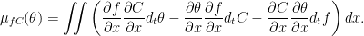
Multiply by a smooth function θ(t, x) and integrate. I denote this by μ_fC(θ). In a stroke of luck, a few applications of integration by parts removes all 2nd derivatives!

We obtain μ_fC(θ) = ∬(f_xC_xθ_t - θ_xf_xC_t - C_xθ_xf_t)dtdx.

➢ Combine partial time derivatives with time integrals to replace with Lebesgue-Stieltjes integrals. I.e., replace f_tdt by d_tf.

As C is convex in x and monotonic in t, it already has x-derivatives almost-everywhere and, by monotonicity, the Lebesgue-Stieltjes integral in t exists. We just need f to also satisfy these properties.

➢ Let’s pause for a moment to consider what the expression μ_fC(θ) really means. As used here, it is just an expression involving 1st order derivatives which vanishes in the event that f(t, X_t) is a martingale. However, it can also be shown to be given by

Alternatively, assuming that f is sufficiently regular that we can decompose f(t, X_t) = M_t + V_t for martingale M and continuous process V of integrable variation (i.e., the drift term) then,

So, μ_fC(θ) is the expected value of the integral of θ(t, X_t) with respect to the drift of f(t, X_t), and the vanishing of this drift is our martingale condition. The fact that this can be expressed only using first order derivatives of f, C and θ is surprising.

➢ If we try to prove that μ_fC = 0 is a valid martingale condition by using the methods of this thread, we must assume that X satisfies the SDE above and f and C are both smooth. Constructing a general proof without imposing smoothness constraints is difficult. I achieved this in the following paper, but required the theory of Dirichlet processes and a time-reversed Doob-Meyer quasimartingale decomposition.

➢ The first step in the proofs, is to identify the class of processes for X to apply the procedure to. It should include solutions to the local vol SDE, but also certain limits of these. It turns out that the suitable properties are that X should be a continuous strong Markov martingale.

➢ I showed that the continuous strong Markov martingale property is preserved under the relevant limits here:

➢ I also showed that if X is of this type the conditional expectations

are sufficiently regular in the following paper.

Specifically, if g is convex then f is convex in x and decreasing in t. So μ_fC is well-defined, and the approach works!

➢ This used coupling techniques introduced by David Hobson here:

Putting together everything described above gives a complete solution. A backwards equation with well-defined solutions guaranteeing uniqueness of the continuous strong Markov martingale X!

➢ The question of existence of strong Markov continuous martingales with given marginals can be answered by taking limits of smooth (or otherwise tractable) marginals, and using the fact that the property is preserved under such limits.

I did this here:

➢ I did allow certain mild kinds of discontinuity for X in my linked papers, to handle those marginals which are inconsistent with a continuous process.

Now that we have existence and uniqueness, we are done!