Figure 1: Brownian motion and its local time surface
The local time of a semimartingale at a level x is a continuous increasing process, giving a measure of the amount of time that the process spends at the given level. As the definition involves stochastic integrals, it was only defined up to probability one. This can cause issues if we want to simultaneously consider local times at all levels. As x can be any real number, it can take uncountably many values and, as a union of uncountably many zero probability sets can have positive measure or, even, be unmeasurable, this is not sufficient to determine the entire local time ‘surface’
for almost all . This is the common issue of choosing good versions of processes. In this case, we already have a continuous version in the time index but, as yet, have not constructed a good version jointly in the time and level. This issue arose in the post on the Ito–Tanaka–Meyer formula, for which we needed to choose a version which is jointly measurable. Although that was sufficient there, joint measurability is still not enough to uniquely determine the full set of local times, up to probability one. The ideal situation is when a version exists which is jointly continuous in both time and level, in which case we should work with this choice. This is always possible for continuous local martingales.
Theorem 1 Let X be a continuous local martingale. Then, the local times
have a modification which is jointly continuous in x and t. Furthermore, this is almost surely -Hölder continuous w.r.t. x, for all and over all bounded regions for t.
Figure 1: Fractional Brownian motion with H = 1/4, 1/2, 3/4
One of the common themes throughout the theory of continuous-time stochastic processes, is the importance of choosing good versions of processes. Specifying the finite distributions of a process is not sufficient to determine its sample paths so, if a continuous modification exists, then it makes sense to work with that. A relatively straightforward criterion ensuring the existence of a continuous version is provided by Kolmogorov’s continuity theorem.
For any positive real number , a map between metric spaces E and F is said to be -Hölder continuous if there exists a positive constant C satisfying
for all . The smallest value of C satisfying this inequality is known as the -Hölder coefficient of . Hölder continuous functions are always continuous and, at least on bounded spaces, is a stronger property for larger values of the coefficient . So, if E is a bounded metric space and , then every -Hölder continuous map from E is also -Hölder continuous. In particular, 1-Hölder and Lipschitz continuity are equivalent.
Kolmogorov’s theorem gives simple conditions on the pairwise distributions of a process which guarantee the existence of a continuous modification but, also, states that the sample paths are almost surely locally Hölder continuous. That is, they are almost surely Hölder continuous on every bounded interval. To start with, we look at real-valued processes. Throughout this post, we work with repect to a probability space . There is no need to assume the existence of any filtration, since they play no part in the results here
Theorem 1 (Kolmogorov) Let be a real-valued stochastic process such that there exists positive constants satisfying
for all . Then, X has a continuous modification which, with probability one, is locally -Hölder continuous for all .
Ito’s lemma is one of the most important and useful results in the theory of stochastic calculus. This is a stochastic generalization of the chain rule, or change of variables formula, and differs from the classical deterministic formulas by the presence of a quadratic variation term. One drawback which can limit the applicability of Ito’s lemma in some situations, is that it only applies for twice continuously differentiable functions. However, the quadratic variation term can alternatively be expressed using local times, which relaxes the differentiability requirement. This generalization of Ito’s lemma was derived by Tanaka and Meyer, and applies to one dimensional semimartingales.
The local time of a stochastic process X at a fixed level x can be written, very informally, as an integral of a Dirac delta function with respect to the continuous part of the quadratic variation ,
(1)
This was explained in an earlier post. As the Dirac delta is only a distribution, and not a true function, equation (1) is not really a well-defined mathematical expression. However, as we saw, with some manipulation a valid expression can be obtained which defines the local time whenever X is a semimartingale.
Going in a slightly different direction, we can try multiplying (1) by a bounded measurable function and integrating over x. Commuting the order of integration on the right hand side, and applying the defining property of the delta function, that is equal to , gives
(2)
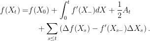
By eliminating the delta function, the right hand side has been transformed into a well-defined expression. In fact, it is now the left side of the identity that is a problem, since the local time was only defined up to probability one at each level x. Ignoring this issue for the moment, recall the version of Ito’s lemma for general non-continuous semimartingales,
(3)
where . Equation (2) allows us to express this quadratic variation term using local times,
The benefit of this form is that, even though it still uses the second derivative of , it is only really necessary for this to exist in a weaker, measure theoretic, sense. Suppose that is convex, or a linear combination of convex functions. Then, its right-hand derivative exists, and is itself of locally finite variation. Hence, the Stieltjes integral exists. The infinitesimal is alternatively written and, in the twice continuously differentiable case, equals . Then,
Fubini’s theorem states that, subject to precise conditions, it is possible to switch the order of integration when computing double integrals. In the theory of stochastic calculus, we also encounter double integrals and would like to be able to commute their order. However, since these can involve stochastic integration rather than the usual deterministic case, the classical results are not always applicable. To help with such cases, we could do with a new stochastic version of Fubini’s theorem. Here, I will consider the situation where one integral is of the standard kind with respect to a finite measure, and the other is stochastic. To start, recall the classical Fubini theorem.
Theorem 1 (Fubini) Let and be finite measure spaces, and be a bounded -measurable function. Then,
Figure 1: Brownian motion B with local time L and auxiliary Brownian motion W
For a stochastic process X taking values in a state space E, its local time at a point is a measure of the time spent at x. For a continuous time stochastic process, we could try and simply compute the Lebesgue measure of the time at the level,
(1)
For processes which hit the level and stick there for some time, this makes some sense. However, if X is a standard Brownian motion, it will always give zero, so is not helpful. Even though X will hit every real value infinitely often, continuity of the normal distribution gives at each positive time, so that that defined by (1) will have zero expectation.
Rather than the indicator function of as in (1), an alternative is to use the Dirac delta function,
(2)
Unfortunately, the Dirac delta is not a true function, it is a distribution, so (2) is not a well-defined expression. However, if it can be made rigorous, then it does seem to have some of the properties we would want. For example, the expectation can be interpreted as the probability density of evaluated at , which has a positive and finite value, so it should lead to positive and finite local times. Equation (2) still relies on the Lebesgue measure over the time index, so will not behave as we may expect under time changes, and will not make sense for processes without a continuous probability density. A better approach is to integrate with respect to the quadratic variation,
(3)
which, for Brownian motion, amounts to the same thing. Although (3) is still not a well-defined expression, since it still involves the Dirac delta, the idea is to come up with a definition which amounts to the same thing in spirit. Important properties that it should satisfy are that it is an adapted, continuous and increasing process with increments supported on the set ,
Local times are a very useful and interesting part of stochastic calculus, and finds important applications to excursion theory, stochastic integration and stochastic differential equations. However, I have not covered this subject in my notes, so do this now. Recalling Ito’s lemma for a function of a semimartingaleX, this involves a term of the form and, hence, requires to be twice differentiable. If we were to try to apply the Ito formula for functions which are not twice differentiable, then can be understood in terms of distributions, and delta functions can appear, which brings local times into the picture. In the opposite direction, which I take in this post, we can try to generalise Ito’s formula and invert this to give a meaning to (3). Continue reading “Semimartingale Local Times”→
In the previous post I introduced the definitions of the dual optional and predictable projections, firstly for processes of integrable variation and, then, generalised to processes which are only required to be locally (or prelocally) of integrable variation. We did not look at the properties of these dual projections beyond the fact that they exist and are uniquely defined, which are significant and important statements in their own right.
To recap, recall that an IV process, A, is right-continuous and such that its variation
(1)
is integrable at time , so that . The dual optional projection is defined for processes which are prelocally IV. That is, A has a dual optional projection if it is right-continuous and its variation process is prelocally integrable, so that there exist a sequence of stopping times increasing to infinity with integrable. More generally, A is a raw FV process if it is right-continuous with almost-surely finite variation over finite time intervals, so (a.s.) for all . Then, if a jointly measurable process is A-integrable on finite time intervals, we use
to denote the integral of with respect to A over the interval , which takes into account the value of at time 0 (unlike the integral which, implicitly, is defined on the interval ). In what follows, whenever we state that has any properties, such as being IV or prelocally IV, we are also including the statement that is A-integrable so that is a well-defined process. Also, whenever we state that a process has a dual optional projection, then we are also implicitly stating that it is prelocally IV.
From theorem 3 of the previous post, the dual optional projection is the unique prelocally IV process satisfying
for all measurable processes with optional projection such that and are IV. Equivalently, is the unique optional FV process such that
for all optional such that is IV, in which case is also IV so that the expectations in this identity are well-defined.
I now look at the elementary properties of dual optional projections, as well as the corresponding properties of dual predictable projections. The most important property is that, according to the definition just stated, the dual projection exists and is uniquely defined. By comparison, the properties considered in this post are elementary and relatively easy to prove. So, I will simply state a theorem consisting of a list of all the properties under consideration, and will then run through their proofs. Starting with the dual optional projection, the main properties are listed below as Theorem 1.
Note that the first three statements are saying that the dual projection is indeed a linear projection from the prelocally IV processes onto the linear subspace of optional FV processes. As explained in the previous post, by comparison with the discrete-time setting, the dual optional projection can be expressed, in a non-rigorous sense, as taking the optional projection of the infinitesimal increments,
(2)
As is interpreted via the Lebesgue-Stieltjes integral, it is a random measure rather than a real-valued process. So, the optional projection of appearing in (2) does not really make sense. However, Theorem 1 does allow us to make sense of (2) in certain restricted cases. For example, if A is differentiable so that for a process , then (9) below gives . This agrees with (2) so long as is interpreted to mean . Also, restricting to the jump component of the increments, , (2) reduces to (11) below.
We defined the dual projection via expectations of integrals with the restriction that this is IV. An alternative approach is to first define the dual projections for IV processes, as was done in theorems 1 and 2 of the previous post, and then extend to (pre)locally IV processes by localisation of the projection. That this is consistent with our definitions follows from the fact that (pre)localisation commutes with the dual projection, as stated in (10) below.
Theorem 1
A raw FV process A is optional if and only if exists and is equal to A.
If the dual optional projection of A exists then,
(3)
If the dual optional projections of A and B exist, and , are -measurable random variables then,
(4)
If the dual optional projection exists then is almost-surely finite and
(5)
If U is a random variable and is a stopping time, then is prelocally IV if and only if is almost surely finite, in which case
(6)
If the prelocally IV process A is nonnegative and increasing then so is and,
(7)
for all nonnegative measurable with optional projection . If A is merely increasing then so is and (7) holds for nonnegative measurable with .
If A has dual optional projection and is an optional process such that is prelocally IV then, is -integrable and,
(8)
If A is an optional FV process and is a measurable process with optional projection such that is prelocally IV then, is A-integrable and,
(9)
If A has dual optional projection and is a stopping time then,
(10)
If the dual optional projection exists, then its jump process is the optional projection of the jump process of A,
(11)
If A has dual optional projection then
(12)
for all nonnegative measurable with optional projection .
Let be a sequence of right-continuous processes with variation
The optional and predictable projections of stochastic processes have corresponding dual projections, which are the subject of this post. I will be concerned with their initial construction here, and show that they are well-defined. The study of their properties will be left until later. In the discrete time setting, the dual projections are relatively straightforward, and can be constructed by applying the optional and predictable projection to the increments of the process. In continuous time, we no longer have discrete time increments along which we can define the dual projections. In some sense, they can still be thought of as projections of the infinitesimal increments so that, for a process A, the increments of the dual projections and are determined from the increments of A as
(1)
Unfortunately, these expressions are difficult to make sense of in general. In specific cases, (1) can be interpreted in a simple way. For example, when A is differentiable with derivative , so that , then the dual projections are given by and . More generally, if A is right-continuous with finite variation, then the infinitesimal increments can be interpreted in terms of Lebesgue-Stieltjes integrals. However, as the optional and predictable projections are defined for real valued processes, and is viewed as a stochastic measure, the right-hand-side of (1) is still problematic. This can be rectified by multiplying by an arbitrary process , and making use of the transitivity property . Integrating over time gives the more meaningful expressions
In contrast to (1), these equalities can be used to give mathematically rigorous definitions of the dual projections. As usual, we work with respect to a complete filtered probability space, and processes are identified whenever they are equal up to evanescence. The terminology `raw IV process‘ will be used to refer to any right-continuous integrable process whose variation on the whole of has finite expectation. The use of the word `raw’ here is just to signify that we are not requiring the process to be adapted. Next, to simplify the expressions, I will use the notation for the integral of a process with respect to another process A,
Note that, whereas the integral is implicitly taken over the range and does not involve the time-zero value of , I have included the time-zero values of the processes in the definition of . This is not essential, and could be excluded, so long as we were to restrict to processes starting from zero. The existence and uniqueness (up to evanescence) of the dual projections is given by the following result.
Theorem 1 (Dual Projections) Let A be a raw IV process. Then,
There exists a unique raw IV process satisfying
(2)
for all bounded measurable processes . We refer to as the dual optional projection of A.
There exists a unique raw IV process satisfying
(3)
for all bounded measurable processes . We refer to as the dual predictable projection of A.
Furthermore, if A is nonnegative and increasing then so are and .
Recall that the the optional and predictable projections of a process are defined, firstly, by a measurability property and, secondly, by their values at stopping times. Namely, the optional projection is measurable with respect to the optional sigma-algebra, and its value is defined at each stopping time by a conditional expectation of the original process. Similarly, the predictable projection is measurable with respect to the predictable sigma-algebra and its value at each predictable stopping time is given by a conditional expectation. While these definitions can be powerful, and many properties of the projections follow immediately, they say very little about the sample paths. Given a stochastic process X defined on a filtered probability space with optional projection then, for each , we may be interested in the sample path . For example, is it continuous, right-continuous, cadlag, etc? Answering these questions requires looking at simultaneously at the uncountable set of times , so the definition of the projection given by specifying its values at each individual stopping time, up to almost-sure equivalence, is not easy to work with. I did establish some of the basic properties of the projections in the previous post, but these do not say much regarding sample paths.
I will now establish the basic properties of the sample paths of the projections. Although these results are quite advanced, most of the work has already been done in these notes when we established some pathwise properties of optional and predictable processes in terms of their behaviour along sequences of stopping times, and of predictable stopping times. So, the proofs in this post are relatively simple and will consist of applications of these earlier results.
Before proceeding, let us consider what kind of properties it is reasonable to expect of the projections. Firstly, it does not seem reasonable to expect the optional projection or the predictable projection to satisfy properties not held by the original process X. Therefore, in this post, we will be concerned with the sample path properties which are preserved by the projections. Consider a process with constant paths. That is, at all times t, for some bounded random variable U. This has about as simple sample paths as possible, so any properties preserved by the projections should hold for the optional and predictable projections of X. However, we know what the projections of this process are. Letting M be the martingale defined by then, assuming that the underlying filtration is right-continuous, M has a cadlag modification and, furthermore, this modification is the optional projection of X. So, assuming that the filtration is right-continuous, the optional projection of X is cadlag, meaning that it is right-continuous and has left limits everywhere. So, we can hope that the optional projection preserves these properties. If the filtration is not right-continuous, then M need not have a cadlag modification, so we cannot expect optional projection to preserve right-continuity in this case. However, M does still have a version with left and right limits everywhere, which is the optional projection of X. So, without assuming right-continuity of the filtration, we may still hope that the optional projection preserves the existence of left and right limits of a process. Next, the predictable projection is equal to the left limits, , which is left-continuous with left and right limits everywhere. Therefore, we can hope that predictable projections preserve left-continuity and the existence of left and right limits. The existence of cadlag martingales which are not continuous, such as the compensated Poisson process, imply that optional projections do not generally preserve left-continuity and the predictable projection does not preserve right-continuity.
Recall that I previously constructed a version of the optional projection and the predictable projection for processes which are, respectively, right-continuous and left-continuous. This was done by defining the projection at each deterministic time and, then, enforcing the respective properties of the sample paths. We can use the results in those posts to infer that the projections do indeed preserve these properties, although I will now more direct proofs in greater generality, and using the more general definition of the optional and predictable projections.
We work with respect to a complete filtered probability space. As usual, we say that the sample paths of a process satisfy any stated property if they satisfy it up to evanescence. Since integrability conditions will be required, I mention those now. Recall that a process X is of class (D) if the set of random variables , over stopping times , is uniformly integrable. It will be said to be locally of class (D) if there is a sequence of stopping times increasing to infinity and such that is of class (D) for each n. Similarly, it will be said to be prelocally of class (D) if there is a sequence of stopping times increasing to infinity and such that is of class (D) for each n.
Theorem 1 Let X be pre-locally of class (D), with optional projection . Then,
if X has left limits, so does .
if X has right limits, so does .
Furthermore, if the underlying filtration is right-continuous then,
Having defined optional and predictable projections in an earlier post, I now look at their basic properties. The first nontrivial property is that they are well-defined in the first place. Recall that existence of the projections made use of the existence of cadlag modifications of martingales, and uniqueness relied on the section theorems. By contrast, once we accept that optional and predictable projections are well-defined, everything in this post follows easily. Nothing here requires any further advanced results of stochastic process theory.
Optional and predictable projections are similar in nature to conditional expectations. Given a probability space and a sub-sigma-algebra , the conditional expectation of an (-measurable) random variable X is a -measurable random variable . This is defined whenever the integrability condition (a.s.) is satisfied, only depends on X up to almost-sure equivalence, and Y is defined up to almost-sure equivalence. That is, a random variable almost surely equal to X has the same conditional expectation as X. Similarly, a random variable almost-surely equal to Y is also a version of the conditional expectation .
The setup with projections of stochastic processes is similar. We start with a filtered probability space, and a (real-valued) stochastic process is a map
which we assume to be jointly-measurable. That is, it is measurable with respect to the Borel sigma-algebra on the image, and the product sigma-algebra on the domain. The optional and predictable sigma-algebras are contained in the product,
We do not have a reference measure on in order to define conditional expectations with respect to and . However, the optional projection and predictable projection play similar roles. Assuming that the necessary integrability properties are satisfied, then the projections exist. Furthermore, the projection only depends on the process Xup to evanescence (i.e., up to a zero probability set), and and are uniquely defined up to evanescence.
In what follows, we work with respect to a complete filtered probability space. Processes are always only considered up to evanescence, so statements involving equalities, inequalities, and limits of processes are only required to hold outside of a zero probability set. When we say that the optional projection of a process exists, we mean that the integrability condition in the definition of the projection is satisfied. Specifically, that is almost surely finite. Similarly for the predictable projection.
The following lemma gives a list of initial properties of the optional projection. Other than the statement involving stopping times, they all correspond to properties of conditional expectations.
Lemma 1
X is optional if and only if exists and is equal to X.
If the optional projection of X exists then,
(1)
If the optional projections of X and Y exist, and are -measurable random variables, then,
(2)
If the optional projection of X exists and U is an optional process then,
(3)
If the optional projection of X exists and is a stopping time then, the optional projection of the stopped process exists and,
(4)
If and the optional projections of X and Y exist then, .
The aim of this post is to give a direct proof of the theorems of measurable projection and measurable section. These are generally regarded as rather difficult results, and proofs often use ideas from descriptive set theory such as analytic sets. I did previously post a proof along those lines on this blog. However, the results can be obtained in a more direct way, which is the purpose of this post. Here, I present relatively self-contained proofs which do not require knowledge of any advanced topics beyond basic probability theory.
The projection theorem states that if is a complete probability space, then the projection of a measurable subset of onto is measurable. To be precise, the condition is that S is in the product sigma-algebra , where denotes the Borel sets in , and the projection map is denoted
Then, measurable projection states that . Although it looks like a very basic property of measurable sets, maybe even obvious, measurable projection is a surprisingly difficult result to prove. In fact, the requirement that the probability space is complete is necessary and, if it is dropped, then need not be measurable. Counterexamples exist for commonly used measurable spaces such as and . This suggests that there is something deeper going on here than basic manipulations of measurable sets.
By definition, if then, for every , there exists a such that . The measurable section theorem — also known as measurable selection — says that this choice can be made in a measurable way. That is, if S is in then there is a measurable section,
It is convenient to extend to the whole of by setting outside of .
Figure 1: A section of a measurable set
The graph of is
The condition that whenever can alternatively be expressed by stating that . This also ensures that is a subset of , and is a section of S on the whole of if and only if .
The results described here can also be used to prove the optional and predictable section theorems which, at first appearances, also seem to be quite basic statements. The section theorems are fundamental to the powerful and interesting theory of optional and predictable projection which is, consequently, generally considered to be a hard part of stochastic calculus. In fact, the projection and section theorems are really not that hard to prove.
Let us consider how one might try and approach a proof of the projection theorem. As with many statements regarding measurable sets, we could try and prove the result first for certain simple sets, and then generalise to measurable sets by use of the monotone class theorem or similar. For example, let denote the collection of all for which . It is straightforward to show that any finite union of sets of the form for and are in . If it could be shown that is closed under taking limits of increasing and decreasing sequences of sets, then the result would follow from the monotone class theorem. Increasing sequences are easily handled — if is a sequence of subsets of then from the definition of the projection map,
If for each n, this shows that the union is again in . Unfortunately, decreasing sequences are much more problematic. If for all then we would like to use something like
(1)
However, this identity does not hold in general. For example, consider the decreasing sequence . Then, for all n, but is empty, contradicting (1). There is some interesting history involved here. In a paper published in 1905, Henri Lebesgue claimed that the projection of a Borel subset of onto is itself measurable. This was based upon mistakenly applying (1). The error was spotted in around 1917 by Mikhail Suslin, who realised that the projection need not be Borel, and lead him to develop the theory of analytic sets.
Actually, there is at least one situation where (1) can be shown to hold. Suppose that for each , the slices
(2)
are compact. For each , the slices give a decreasing sequence of nonempty compact sets, so has nonempty intersection. So, letting S be the intersection , the slice is nonempty. Hence, , and (1) follows.
The starting point for our proof of the projection and section theorems is to consider certain special subsets of where the compactness argument, as just described, can be used. The notation is used to represent the collection of countable intersections, , of sets in .
Lemma 1 Let be a measurable space, and be the collection of subsets of which are finite unions over compact intervals and . Then, for any , we have , and the debut


-Hölder continuous w.r.t. x, for all
and over all bounded regions for t.


 between metric spaces E and F is said to be
 . The smallest value of C satisfying this inequality is known as the
  . Hölder continuous functions are always continuous and, at least on bounded spaces, is a stronger property for larger values of the coefficient
  , then every
  -Hölder continuous map from E is also
  -Hölder continuous. In particular, 1-Hölder and Lipschitz continuity are equivalent.
 are almost surely locally Hölder continuous. That is, they are almost surely Hölder continuous on every bounded interval. To start with, we look at real-valued processes. Throughout this post, we work with repect to a probability space
  . There is no need to assume the existence of any filtration, since they play no part in the results here
 be a real-valued stochastic process such that there exists positive constants
  satisfying
 ![\displaystyle {\mathbb E}\left[\lvert X_t-X_s\rvert^\alpha\right]\le C\lvert t-s\vert^{1+\beta},](https://s0.wp.com/latex.php?latex=%5Cdisplaystyle++%7B%5Cmathbb+E%7D%5Cleft%5B%5Clvert+X_t-X_s%5Crvert%5E%5Calpha%5Cright%5D%5Cle+C%5Clvert+t-s%5Cvert%5E%7B1%2B%5Cbeta%7D%2C+&bg=ffffff&fg=000000&s=0&c=20201002)
 . Then, X has a continuous modification which, with probability one, is locally
  .
. ![{[X]^{c}}](https://s0.wp.com/latex.php?latex=%7B%5BX%5D%5E%7Bc%7D%7D&bg=ffffff&fg=000000&s=0&c=20201002) ,
,![\displaystyle L^x_t=\int_0^t\delta(X-x)d[X]^c.](https://s0.wp.com/latex.php?latex=%5Cdisplaystyle++L%5Ex_t%3D%5Cint_0%5Et%5Cdelta%28X-x%29d%5BX%5D%5Ec.+&bg=ffffff&fg=000000&s=0&c=20201002)
 and integrating over x. Commuting the order of integration on the right hand side, and applying the defining property of the delta function, that
 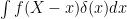 is equal to
  , gives
![\displaystyle \int_{-\infty}^{\infty} L^x_t f(x)dx=\int_0^tf(X)d[X]^c.](https://s0.wp.com/latex.php?latex=%5Cdisplaystyle++%5Cint_%7B-%5Cinfty%7D%5E%7B%5Cinfty%7D+L%5Ex_t+f%28x%29dx%3D%5Cint_0%5Etf%28X%29d%5BX%5D%5Ec.+&bg=ffffff&fg=000000&s=0&c=20201002)
![{A_t=\int_0^t f^{\prime\prime}(X)d[X]^c}](https://s0.wp.com/latex.php?latex=%7BA_t%3D%5Cint_0%5Et+f%5E%7B%5Cprime%5Cprime%7D%28X%29d%5BX%5D%5Ec%7D&bg=ffffff&fg=000000&s=0&c=20201002) . Equation (
. Equation (
 exists, and is itself of locally finite variation. Hence, the Stieltjes integral
  exists. The infinitesimal
  is alternatively written
  and, in the twice continuously differentiable case, equals
  . Then,
 and
and  be finite measure spaces, and
  be a bounded
  -measurable function. Then,
 -measurable,
 -measurable, and,

 is a measure of the time spent at x. For a continuous time stochastic process, we could try and simply compute the Lebesgue measure of the time at the level,
 and stick there for some time, this makes some sense. However, if X is a standard
  at each positive time, so that that
  defined by (
 as in (
![{{\mathbb E}[\delta(X_s-x)]}](https://s0.wp.com/latex.php?latex=%7B%7B%5Cmathbb+E%7D%5B%5Cdelta%28X_s-x%29%5D%7D&bg=ffffff&fg=000000&s=0&c=20201002) can be interpreted as the probability density of
can be interpreted as the probability density of  evaluated at
 ![\displaystyle L^x_t=\int_0^t\delta(X_s-x)d[X]_s](https://s0.wp.com/latex.php?latex=%5Cdisplaystyle++L%5Ex_t%3D%5Cint_0%5Et%5Cdelta%28X_s-x%29d%5BX%5D_s+&bg=ffffff&fg=000000&s=0&c=20201002)

![{\int f^{\prime\prime}(X)d[X]}](https://s0.wp.com/latex.php?latex=%7B%5Cint+f%5E%7B%5Cprime%5Cprime%7D%28X%29d%5BX%5D%7D&bg=ffffff&fg=000000&s=0&c=20201002) and, hence, requires
and, hence, requires  can be understood in terms of distributions, and delta functions can appear, which brings local times into the picture. In the opposite direction, which I take in this post, we can try to generalise Ito’s formula and invert this to give a meaning to (
 , so that
 ![{{\mathbb E}[V_\infty] < \infty}](https://s0.wp.com/latex.php?latex=%7B%7B%5Cmathbb+E%7D%5BV_%5Cinfty%5D+%3C+%5Cinfty%7D&bg=ffffff&fg=000000&s=0&c=20201002) . The dual optional projection is defined for processes which are prelocally IV. That is, A has a dual optional projection
. The dual optional projection is defined for processes which are prelocally IV. That is, A has a dual optional projection  if it is right-continuous and its variation process is prelocally integrable, so that there exist a sequence
  of
of  integrable. More generally, A is a raw FV process if it is right-continuous with almost-surely finite variation over finite time intervals, so
  (a.s.) for all
  . Then, if a jointly measurable process
  is A-integrable on finite time intervals, we use
![{[0,t]}](https://s0.wp.com/latex.php?latex=%7B%5B0%2Ct%5D%7D&bg=ffffff&fg=000000&s=0&c=20201002) , which takes into account the value of
, which takes into account the value of  which, implicitly, is defined on the interval
 ![{(0,t]}](https://s0.wp.com/latex.php?latex=%7B%280%2Ct%5D%7D&bg=ffffff&fg=000000&s=0&c=20201002) ). In what follows, whenever we state that
). In what follows, whenever we state that  has any properties, such as being IV or prelocally IV, we are also including the statement that
 ![\displaystyle {\mathbb E}[\xi\cdot A^{\rm o}_\infty]={\mathbb E}[{}^{\rm o}\xi\cdot A_\infty]](https://s0.wp.com/latex.php?latex=%5Cdisplaystyle++%7B%5Cmathbb+E%7D%5B%5Cxi%5Ccdot+A%5E%7B%5Crm+o%7D_%5Cinfty%5D%3D%7B%5Cmathbb+E%7D%5B%7B%7D%5E%7B%5Crm+o%7D%5Cxi%5Ccdot+A_%5Cinfty%5D+&bg=ffffff&fg=000000&s=0&c=20201002)
 such that
  and
and  are IV. Equivalently,
 ![\displaystyle {\mathbb E}[\xi\cdot A^{\rm o}_\infty]={\mathbb E}[\xi\cdot A_\infty]](https://s0.wp.com/latex.php?latex=%5Cdisplaystyle++%7B%5Cmathbb+E%7D%5B%5Cxi%5Ccdot+A%5E%7B%5Crm+o%7D_%5Cinfty%5D%3D%7B%5Cmathbb+E%7D%5B%5Cxi%5Ccdot+A_%5Cinfty%5D+&bg=ffffff&fg=000000&s=0&c=20201002)

 is interpreted via the
  , it is a random measure rather than a real-valued process. So, the optional projection of
  for a process
  . This agrees with (
 is interpreted to mean
  . Also, restricting to the jump component of the increments,
  , (
, (
 ,
,  are
are  -measurable random variables then,
![{{\mathbb E}[\lvert A_0\rvert\,\vert\mathcal F_0]}](https://s0.wp.com/latex.php?latex=%7B%7B%5Cmathbb+E%7D%5B%5Clvert+A_0%5Crvert%5C%2C%5Cvert%5Cmathcal+F_0%5D%7D&bg=ffffff&fg=000000&s=0&c=20201002) is almost-surely finite and
is almost-surely finite and![\displaystyle A^{\rm o}_0={\mathbb E}[A_0\,\vert\mathcal F_0].](https://s0.wp.com/latex.php?latex=%5Cdisplaystyle++A%5E%7B%5Crm+o%7D_0%3D%7B%5Cmathbb+E%7D%5BA_0%5C%2C%5Cvert%5Cmathcal+F_0%5D.+&bg=ffffff&fg=000000&s=0&c=20201002)
 is a stopping time, then
  is prelocally IV if and only if
 ![{{\mathbb E}[1_{\{\tau < \infty\}}\lvert U\rvert\,\vert\mathcal F_\tau]}](https://s0.wp.com/latex.php?latex=%7B%7B%5Cmathbb+E%7D%5B1_%7B%5C%7B%5Ctau+%3C+%5Cinfty%5C%7D%7D%5Clvert+U%5Crvert%5C%2C%5Cvert%5Cmathcal+F_%5Ctau%5D%7D&bg=ffffff&fg=000000&s=0&c=20201002) is almost surely finite, in which case
is almost surely finite, in which case![\displaystyle \left(U1_{[\tau,\infty)}\right)^{\rm o}={\mathbb E}[1_{\{\tau < \infty\}}U\,\vert\mathcal F_\tau]1_{[\tau,\infty)}.](https://s0.wp.com/latex.php?latex=%5Cdisplaystyle++%5Cleft%28U1_%7B%5B%5Ctau%2C%5Cinfty%29%7D%5Cright%29%5E%7B%5Crm+o%7D%3D%7B%5Cmathbb+E%7D%5B1_%7B%5C%7B%5Ctau+%3C+%5Cinfty%5C%7D%7DU%5C%2C%5Cvert%5Cmathcal+F_%5Ctau%5D1_%7B%5B%5Ctau%2C%5Cinfty%29%7D.+&bg=ffffff&fg=000000&s=0&c=20201002)
 .
. 


![\displaystyle \setlength\arraycolsep{2pt} \begin{array}{rl} &\displaystyle{\mathbb E}\left[\xi_0\lvert A^{\rm o}_0\rvert + \int_0^\infty\xi\,\lvert dA^{\rm o}\rvert\right]\le{\mathbb E}\left[{}^{\rm o}\xi_0\lvert A_0\rvert + \int_0^\infty{}^{\rm o}\xi\,\lvert dA\rvert\right],\smallskip\\ &\displaystyle{\mathbb E}\left[\xi_0(A^{\rm o}_0)_+ + \int_0^\infty\xi\,(dA^{\rm o})_+\right]\le{\mathbb E}\left[{}^{\rm o}\xi_0(A_0)_+ + \int_0^\infty{}^{\rm o}\xi\,(dA)_+\right],\smallskip\\ &\displaystyle{\mathbb E}\left[\xi_0(A^{\rm o}_0)_- + \int_0^\infty\xi\,(dA^{\rm o})_-\right]\le{\mathbb E}\left[{}^{\rm o}\xi_0(A_0)_- + \int_0^\infty{}^{\rm o}\xi\,(dA)_-\right], \end{array}](https://s0.wp.com/latex.php?latex=%5Cdisplaystyle++%5Csetlength%5Carraycolsep%7B2pt%7D+%5Cbegin%7Barray%7D%7Brl%7D+%26%5Cdisplaystyle%7B%5Cmathbb+E%7D%5Cleft%5B%5Cxi_0%5Clvert+A%5E%7B%5Crm+o%7D_0%5Crvert+%2B+%5Cint_0%5E%5Cinfty%5Cxi%5C%2C%5Clvert+dA%5E%7B%5Crm+o%7D%5Crvert%5Cright%5D%5Cle%7B%5Cmathbb+E%7D%5Cleft%5B%7B%7D%5E%7B%5Crm+o%7D%5Cxi_0%5Clvert+A_0%5Crvert+%2B+%5Cint_0%5E%5Cinfty%7B%7D%5E%7B%5Crm+o%7D%5Cxi%5C%2C%5Clvert+dA%5Crvert%5Cright%5D%2C%5Csmallskip%5C%5C+%26%5Cdisplaystyle%7B%5Cmathbb+E%7D%5Cleft%5B%5Cxi_0%28A%5E%7B%5Crm+o%7D_0%29_%2B+%2B+%5Cint_0%5E%5Cinfty%5Cxi%5C%2C%28dA%5E%7B%5Crm+o%7D%29_%2B%5Cright%5D%5Cle%7B%5Cmathbb+E%7D%5Cleft%5B%7B%7D%5E%7B%5Crm+o%7D%5Cxi_0%28A_0%29_%2B+%2B+%5Cint_0%5E%5Cinfty%7B%7D%5E%7B%5Crm+o%7D%5Cxi%5C%2C%28dA%29_%2B%5Cright%5D%2C%5Csmallskip%5C%5C+%26%5Cdisplaystyle%7B%5Cmathbb+E%7D%5Cleft%5B%5Cxi_0%28A%5E%7B%5Crm+o%7D_0%29_-+%2B+%5Cint_0%5E%5Cinfty%5Cxi%5C%2C%28dA%5E%7B%5Crm+o%7D%29_-%5Cright%5D%5Cle%7B%5Cmathbb+E%7D%5Cleft%5B%7B%7D%5E%7B%5Crm+o%7D%5Cxi_0%28A_0%29_-+%2B+%5Cint_0%5E%5Cinfty%7B%7D%5E%7B%5Crm+o%7D%5Cxi%5C%2C%28dA%29_-%5Cright%5D%2C+%5Cend%7Barray%7D+&bg=ffffff&fg=000000&s=0&c=20201002)
 be a sequence of right-continuous processes with variation

 is prelocally IV then,
 are determined from the increments
 , then the dual projections are given by
  and
and  . More generally, if A is right-continuous with finite variation, then the infinitesimal increments
 ![{{\mathbb E}[\xi\,{}^{\rm o}(dA)]={\mathbb E}[({}^{\rm o}\xi)dA]}](https://s0.wp.com/latex.php?latex=%7B%7B%5Cmathbb+E%7D%5B%5Cxi%5C%2C%7B%7D%5E%7B%5Crm+o%7D%28dA%29%5D%3D%7B%5Cmathbb+E%7D%5B%28%7B%7D%5E%7B%5Crm+o%7D%5Cxi%29dA%5D%7D&bg=ffffff&fg=000000&s=0&c=20201002) . Integrating over time gives the more meaningful expressions
. Integrating over time gives the more meaningful expressions ![\displaystyle \setlength\arraycolsep{2pt} \begin{array}{rl} &\displaystyle {\mathbb E}\left[\int_0^\infty \xi\,dA^{\rm o}\right]={\mathbb E}\left[\int_0^\infty{}^{\rm o}\xi\,dA\right],\smallskip\\ &\displaystyle{\mathbb E}\left[\int_0^\infty \xi\,dA^{\rm p}\right]={\mathbb E}\left[\int_0^\infty{}^{\rm p}\xi\,dA\right]. \end{array}](https://s0.wp.com/latex.php?latex=%5Cdisplaystyle++%5Csetlength%5Carraycolsep%7B2pt%7D+%5Cbegin%7Barray%7D%7Brl%7D+%26%5Cdisplaystyle+%7B%5Cmathbb+E%7D%5Cleft%5B%5Cint_0%5E%5Cinfty+%5Cxi%5C%2CdA%5E%7B%5Crm+o%7D%5Cright%5D%3D%7B%5Cmathbb+E%7D%5Cleft%5B%5Cint_0%5E%5Cinfty%7B%7D%5E%7B%5Crm+o%7D%5Cxi%5C%2CdA%5Cright%5D%2C%5Csmallskip%5C%5C+%26%5Cdisplaystyle%7B%5Cmathbb+E%7D%5Cleft%5B%5Cint_0%5E%5Cinfty+%5Cxi%5C%2CdA%5E%7B%5Crm+p%7D%5Cright%5D%3D%7B%5Cmathbb+E%7D%5Cleft%5B%5Cint_0%5E%5Cinfty%7B%7D%5E%7B%5Crm+p%7D%5Cxi%5C%2CdA%5Cright%5D.+%5Cend%7Barray%7D+&bg=ffffff&fg=000000&s=0&c=20201002)
 , and processes are identified whenever they are equal
  has finite expectation. The use of the word `raw’ here is just to signify that we are not requiring the process to be
![\displaystyle {\mathbb E}\left[\xi\cdot A^{\rm o}_\infty\right]={\mathbb E}\left[{}^{\rm o}\xi\cdot A_\infty\right]](https://s0.wp.com/latex.php?latex=%5Cdisplaystyle++%7B%5Cmathbb+E%7D%5Cleft%5B%5Cxi%5Ccdot+A%5E%7B%5Crm+o%7D_%5Cinfty%5Cright%5D%3D%7B%5Cmathbb+E%7D%5Cleft%5B%7B%7D%5E%7B%5Crm+o%7D%5Cxi%5Ccdot+A_%5Cinfty%5Cright%5D+&bg=ffffff&fg=000000&s=0&c=20201002)
![\displaystyle {\mathbb E}\left[\xi\cdot A^{\rm p}_\infty\right]={\mathbb E}\left[{}^{\rm p}\xi\cdot A_\infty\right]](https://s0.wp.com/latex.php?latex=%5Cdisplaystyle++%7B%5Cmathbb+E%7D%5Cleft%5B%5Cxi%5Ccdot+A%5E%7B%5Crm+p%7D_%5Cinfty%5Cright%5D%3D%7B%5Cmathbb+E%7D%5Cleft%5B%7B%7D%5E%7B%5Crm+p%7D%5Cxi%5Ccdot+A_%5Cinfty%5Cright%5D+&bg=ffffff&fg=000000&s=0&c=20201002)
 then, for each
  . For example, is it continuous, right-continuous,
  simultaneously at the uncountable set of times
  to satisfy properties not held by the original process X. Therefore, in this post, we will be concerned with the sample path properties which are preserved by the projections. Consider a process with constant paths. That is,
  at all times t, for some bounded random variable U. This has about as simple sample paths as possible, so any properties preserved by the projections should hold for the optional and predictable projections of X. However, we know what
 ![{M_t={\mathbb E}[U\,\vert\mathcal F_t]}](https://s0.wp.com/latex.php?latex=%7BM_t%3D%7B%5Cmathbb+E%7D%5BU%5C%2C%5Cvert%5Cmathcal+F_t%5D%7D&bg=ffffff&fg=000000&s=0&c=20201002) then, assuming that the underlying filtration is right-continuous, M has a
then, assuming that the underlying filtration is right-continuous, M has a  , which is left-continuous with left and right limits everywhere. Therefore, we can hope that predictable projections preserve left-continuity and the existence of left and right limits. The existence of cadlag martingales which are not continuous, such as the
  , over stopping times
 ![{1_{\{\tau_n > 0\}}1_{[0,\tau_n]}X}](https://s0.wp.com/latex.php?latex=%7B1_%7B%5C%7B%5Ctau_n+%3E+0%5C%7D%7D1_%7B%5B0%2C%5Ctau_n%5D%7DX%7D&bg=ffffff&fg=000000&s=0&c=20201002) is of class (D) for each n. Similarly, it will be said to be prelocally of class (D) if there is a sequence
is of class (D) for each n. Similarly, it will be said to be prelocally of class (D) if there is a sequence  is of class (D) for each n.
 and a sub-sigma-algebra
  , the conditional expectation of an (
 -measurable random variable
 ![{Y={\mathbb E}[X\,\vert\mathcal G]}](https://s0.wp.com/latex.php?latex=%7BY%3D%7B%5Cmathbb+E%7D%5BX%5C%2C%5Cvert%5Cmathcal+G%5D%7D&bg=ffffff&fg=000000&s=0&c=20201002) . This is defined whenever the integrability condition
. This is defined whenever the integrability condition ![{{\mathbb E}[\lvert X\rvert\,\vert\mathcal G] < \infty}](https://s0.wp.com/latex.php?latex=%7B%7B%5Cmathbb+E%7D%5B%5Clvert+X%5Crvert%5C%2C%5Cvert%5Cmathcal+G%5D+%3C+%5Cinfty%7D&bg=ffffff&fg=000000&s=0&c=20201002) (a.s.) is satisfied, only depends on X up to almost-sure equivalence, and Y is defined up to almost-sure equivalence. That is, a random variable
(a.s.) is satisfied, only depends on X up to almost-sure equivalence, and Y is defined up to almost-sure equivalence. That is, a random variable  almost surely equal to X has the same conditional expectation as X. Similarly, a random variable
  almost-surely equal to Y is also a version of the conditional expectation
 ![{{\mathbb E}[X\,\vert\mathcal G]}](https://s0.wp.com/latex.php?latex=%7B%7B%5Cmathbb+E%7D%5BX%5C%2C%5Cvert%5Cmathcal+G%5D%7D&bg=ffffff&fg=000000&s=0&c=20201002) .
.

 on the image, and the product sigma-algebra
  on the domain. The optional and predictable sigma-algebras are contained in the product,
 in order to define conditional expectations with respect to
  and
and  . However, the optional projection
 ![{{\mathbb E}[1_{\{\tau < \infty\}}\lvert X_\tau\rvert\,\vert\mathcal F_\tau]}](https://s0.wp.com/latex.php?latex=%7B%7B%5Cmathbb+E%7D%5B1_%7B%5C%7B%5Ctau+%3C+%5Cinfty%5C%7D%7D%5Clvert+X_%5Ctau%5Crvert%5C%2C%5Cvert%5Cmathcal+F_%5Ctau%5D%7D&bg=ffffff&fg=000000&s=0&c=20201002) is almost surely finite. Similarly for the predictable projection.
is almost surely finite. Similarly for the predictable projection.

 are
are  -measurable random variables, then,
 exists and,
![\displaystyle 1_{[0,\tau]}{}^{\rm o}(X^\tau)=1_{[0,\tau]}{}^{\rm o}\!X.](https://s0.wp.com/latex.php?latex=%5Cdisplaystyle++1_%7B%5B0%2C%5Ctau%5D%7D%7B%7D%5E%7B%5Crm+o%7D%28X%5E%5Ctau%29%3D1_%7B%5B0%2C%5Ctau%5D%7D%7B%7D%5E%7B%5Crm+o%7D%5C%21X.+&bg=ffffff&fg=000000&s=0&c=20201002)
 and the optional projections of X and Y exist then,
  .
.
 onto
onto  is measurable. To be precise, the condition is that S is in the product sigma-algebra
  , and the projection map is denoted
 . Although it looks like a very basic property of measurable sets, maybe even obvious, measurable projection is a surprisingly difficult result to prove. In fact, the requirement that the probability space is complete is necessary and, if it is dropped, then
  need not be measurable. Counterexamples exist for commonly used measurable spaces such as
  and
and  . This suggests that there is something deeper going on here than basic manipulations of measurable sets.
 then, for every
  , there exists a
  such that
  . The measurable section theorem — also known as measurable selection — says that this choice can be made in a measurable way. That is, if S is in
 outside of
![\displaystyle [\tau]=\left\{(t,\omega)\in{\mathbb R}\times\Omega\colon t=\tau(\omega)\right\}.](https://s0.wp.com/latex.php?latex=%5Cdisplaystyle++%5B%5Ctau%5D%3D%5Cleft%5C%7B%28t%2C%5Comega%29%5Cin%7B%5Cmathbb+R%7D%5Ctimes%5COmega%5Ccolon+t%3D%5Ctau%28%5Comega%29%5Cright%5C%7D.+&bg=ffffff&fg=000000&s=0&c=20201002)
 whenever
  can alternatively be expressed by stating that
 ![{[\tau]\subseteq S}](https://s0.wp.com/latex.php?latex=%7B%5B%5Ctau%5D%5Csubseteq+S%7D&bg=ffffff&fg=000000&s=0&c=20201002) . This also ensures that
. This also ensures that  is a subset of
  .
. denote the collection of all
  . It is straightforward to show that any finite union of sets of the form
  for
for  and
and  are in
  is a sequence of subsets of
 for each n, this shows that the union
  is again in
  for all
  then we would like to use something like
 . Then,
  for all n, but
  is empty, contradicting (
 onto
onto 
 , the slices
  give a decreasing sequence of nonempty compact sets, so has nonempty intersection. So, letting S be the intersection
  is nonempty. Hence,
  is used to represent the collection of countable intersections,
  , of sets
  in
in  .
. be a measurable space, and
  over compact intervals
  and
and  . Then, for any
  , we have
