The Gaussian Correlation Inequality

When I first created this blog, the subject of my initial post was the Gaussian correlation conjecture. Using to denote the standard n-dimensional Gaussian probability measure, the conjecture states that the inequality

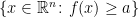
holds for all symmetric convex subsets A and B of . By symmetric, we mean symmetric about the origin, so that is in A if and only is in A, and similarly for B. The standard Gaussian measure by definition has zero mean and covariance matrix equal to the nxn identity matrix, so that

with denoting the Lebesgue integral on . However, if it holds for the standard Gaussian measure, then the inequality can also be shown to hold for any centered (i.e., zero mean) Gaussian measure.

At the time of my original post, the Gaussian correlation conjecture was an unsolved mathematical problem, originally arising in the 1950s and formulated in its modern form in the 1970s. However, in the period since that post, the conjecture has been solved! A proof was published by Thomas Royen in 2014 [7]. This seems to have taken some time to come to the notice of much of the mathematical community. In December 2015, Rafał Latała, and Dariusz Matlak published a simplified version of Royen’s proof [4]. Although the original proof by Royen was already simple enough, it did consider a generalisation of the conjecture to a kind of multivariate gamma distribution. The exposition by Latała and Matlak ignores this generality and adds in some intermediate lemmas in order to improve readability and accessibility. Since then, the result has become widely known and, recently, has even been reported in the popular press [10,11]. There is an interesting article on Royen’s discovery of his proof at Quanta Magazine [12] including the background information that Royen was a 67 year old German retiree who supposedly came up with the idea while brushing his teeth one morning. Dick Lipton and Ken Regan have recently written about the history and eventual solution of the conjecture on their blog [5]. As it has now been shown to be true, I will stop referring to the result as a `conjecture’ and, instead, use the common alternative name — the Gaussian correlation inequality.

In this post, I will describe some equivalent formulations of the Gaussian correlation inequality, or GCI for short, before describing a general method of attacking this problem which has worked for earlier proofs of special cases. I will then describe Royen’s proof and we will see that it uses the same ideas, but with some key differences.

Probably the most surprising aspect of Royen’s proof is its simplicity. Although it does involve some clever algebraic manipulations, no particularly complex mathematics is required to understand it. It seems incredible that a result which has been outstanding for so long has such a simple solution which has eluded all previous attempts. A common approach to the problem is to look at a local version of it and, by taking derivatives, replace it with a more easily manageable statement which I describe below in inequality (11). This `local’ inequality has successfully been used before to prove special cases of GCI, such the 2-dimensional version. Royen’s approach to the problem is similar and, although he does not rely on inequality (11), we will see that (11) does follow indirectly from his proof. So, it seems that the methods which have been used long before Royen published his paper were already along the correct lines but, previously, no-one had quite managed to get it to work. It is intriguing that nobody has produced a direct proof of inequality (11) — to my knowledge, at least.

There are various different, but similar, formulations of GCI, and one of the key steps in Royen’s solution is to start with the correct formulation. I will first describe some of the alternative formulations of the inequality. As above, using to denote the standard Gaussian measure on , GCI states that

(1)

for any symmetric convex sets . In one dimension this is trivial, since the sets will be symmetric intervals, so that one contains the other. So, for , (1) holds with the right hand side replaced by the larger quantity . In dimension , the inequality is already rather difficult to establish, and a proof was first published in 1977 by Pitt [6]. For dimension , no proof of (1) was known prior to Royen’s 2014 paper.

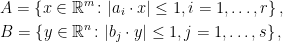
An alternative formulation can be given in terms of probabilities of multidimensional Gaussian random variables lying in specified sets. If are zero-mean jointly Gaussian random vectors taking values in and respectively then,

(2)

for any symmetric convex sets and . This is the form in which the inequality was stated by Da Gupta et al [1], in 1972, in one of the earliest statements of the general conjecture. Inequality (2) is a clear generalization of (1), and reduces to it in the special case with and where are standard Gaussian (i.e., with probability measure ). It can be shown without much trouble that (1) and (2) are equivalent statements. I will leave the proof of this for now, and show that the various formulations of GCI are equivalent in a moment. Dividing through by , inequality (2) can be expressed in terms of conditional probabilities,

So, regardless of the correlations between X and Y, the knowledge that Y is in B increases the probability of finding X in A.

GCI can also be expressed using expectations rather than probabilities. A function is quasiconcave if for all the set is convex. Equivalently,

for all and . For example, indicator functions of convex sets are quasiconcave. If, as above, X and Y are zero-mean jointly Gaussian random vectors taking values in and respectively, then

(3)

for all symmetric quasiconcave functions and . For the specific case where and are indicator functions of sets A and B, (3) reduces to (2). The formulation of GCI given by (3) is expressed by the statement that and have nonnegative covariance.

The final formulation of GCI which I will describe here is expressed in terms of the probabilities that a sequence of Gaussian random variables lie in specified symmetric intervals of . If are zero-mean jointly Gaussian real random variables then,

(4)

for . This formulation is a special case of (2) applied to the sets and ,

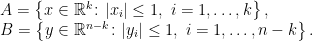(5)

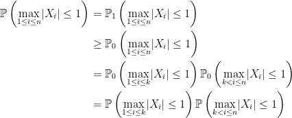
The formulation given by (4) is central to Royen’s proof, but has also been a common form in which the inequality has been stated ever since it was first formulated. The case with was proven in 1967 by both Khatri [3] and Sidak [8]. There is one minor technicality which I glossed over in the statements above. I merely required A and B to be symmetric and convex sets but, for the probabilities to be well-defined, the sets should be measurable. Often the additional requirement that they are closed sets is used, ensuring Borel measurability. However, it is not difficult to show that for any symmetric convex set A with closure , the difference is contained in a set of zero probability with respect to a centered Gaussian measure. Hence, A is already guaranteed to be measurable under the completion of the measure. Furthermore, statements (1) and (2) are unchanged if A and B are replaced by their closures and . Similarly, in (3), I did not require the functions to be measurable but, by quasiconcavity, they are guaranteed to be measurable under the completion of the probability measure.

As promised, we show that each of the alternative formulations of GCI given above are equivalent.

Lemma 1 Each of the forms of GCI given by (1), (2), (3) and (4) are equivalent.

To be precise, here we mean that each of the inequalities are equivalent when stated in their full generality. That is, if any one holds in all dimensions m and n and for all pairs of symmetric convex sets (or quasiconcave functions), then all of the other statements hold.

Equivalence of (1) and (2): It was already noted above that inequality (1) is a special case of (2), so just the reverse implication remains to be shown. That is, assuming that inequality (1) holds, we need to prove (2). To do this, use the standard result that any centered multidimensional Gaussian vector can be expressed as a linear function of a standard Gaussian vector. In our case, this means that there is a random vector Z taking values in (for some k), with the standard Gaussian distribution , and such that and for mxk and nxk matrices M, N. Then,

Applying inequality (1),

as required.

Equivalence of (2) and (3): As (2) is the special case of (3) where are indicator functions of symmetric convex sets, we only need to show that inequality (2) implies (3). We can decompose and as integrals of indicator functions of symmetric convex sets,

(6)

Multiplying these, taking expectations, and using Fubini’s theorem to commute the integrals with the expectation,

Applying inequality (2),

as required.

Equivalence of (2) and (4): It was noted above that (4) is a special case of (2) where the sets A and B are of the form given in equation (5). It only remains to show that inequality (2) follows from the assumption that (4) holds.

Consider the case where and are symmetric convex polytopes. These are convex sets of the form

(7)

for some , and . Defining the joint Gaussian random variables and ,

Applying inequality (4) to this,

This proves (2) for symmetric convex polytopes. It is a consequence of the hyperplane separation theorem that every nonempty symmetric closed convex set is the intersection of a countable sequence of strips of the form and, hence, is the limit of a decreasing sequence of symmetric convex polytopes. This proves (2) for symmetric closed convex sets. Finally, as was mentioned above, inequality (2) is unchanged if the sets A and B are replaced by their closures, extending (2) to all symmetric convex sets.

---

The Local Approach

One method of attacking the Gaussian correlation inequality is to note that both sides of the inequality can be expressed as the values of some function evaluated at different points of a connected topological space. If it can shown that we can move from one of the points to the other, along a continuous path in the space on which the function is monotonic, then GCI would follow. I will describe this approach now.

Let us start with a pair of independent n-dimensional random vectors X and Y, each with the standard Gaussian distribution . Inequality (1) can be written as

(8)

for symmetric convex . If we can continuously transform the pair into in such a way that the probability of being in is increasing, then (8) will follow. A straightforward method is to define

over . Then, has the standard Gaussian distribution for each t with, and . Note that the covariance matrix

is just . Throughout this post I use the term `increasing’ in the non-strict sense, equivalent to `nondecreasing’.

Conjecture C1 For any symmetric convex sets , the probability

(9)

is increasing in t, over the range .

If true, conjecture C1 implies (8) and, hence, the Gaussian correlation inequality. Due to Sidak [9], this conjecture is known to be true if A is a symmetric slab of the form

for some and, from Pitt [6], is true in dimension . Although this conjecture is not used by Royen in his 2014 proof of GCI [7], we will see that it does follow from his argument.

One way of directly trying to prove conjecture C1 is to differentiate (9) with respect to t and show that the result is positive. This is more easily done if the indicator functions , are replaced by differentiable functions. If are continuously differentiable with bounded derivative, a straightforward application of integration by parts gives

(10)

Here denotes the partial derivative with respect to the i‘th component of x. By approximating with smooth functions, it can be seen that (10) holds for arbitrary Lipschitz continuous , which, by Radamacher’s theorem, is sufficient to guarantee that they are differentiable almost everywhere. We want to show that (10) is non-negative. As I will show in a moment, if it always holds at then it will also hold at . As X has distribution , we arrive at the following conjecture.

Conjecture C2 Let be symmetric quasiconcave and Lipschitz continuous functions. Then,

(11)

where is the standard Gaussian measure on .

Inequality (11) was used by Pitt to prove GCI in two dimensions, and appears as Theorem 1 of his 1977 paper [6]. In fact, it is shown that if is a nonnegative decreasing function of then

(12)

The special case with equal to the Gaussian density is equivalent to inequality (11). As stated by Pitt, his proof of (12) does not extend to greater than 2 dimensions but, if it could be extended to then GCI would follow. It seems unlikely that it extends in this generality to three or more dimensions, unless is restricted to being the Gaussian density. Although Royen does not consider this inequality, we will see that (11) is a consequence of his proof. It is interesting that no-one has produced a direct proof of conjecture C2, which could then be used as an alternative proof of GCI.

Conjecture C1 can be stated in a more general form, which I will do now. Letting X and Y be centered Gaussian random vectors of dimension m and n, use and to denote their respective covariance matrices. Consider the (m+n)x(m+n) matrices of the form

Here, Q is any mxn matrix. When is positive semidefinite, let denote a probability measure for which is a centered Gaussian random vector with correlation matrix . Inequality (2) can be written as,

(13)

The first equality here follows because the vectors X and Y have covariance matrices and respectively, so their distribution does not depend on Q. Hence, Q can be replaced by the zero matrix. The second equality holds because, under , X and Y are independent. This shows that GCI is equivalent to stating that

has a global minimum at .

Inequality (13) would be proved if we can find a continuous curve, joining 0 to an arbitrary such that is positive semidefinite and is increasing in t. A similar approach was, in effect, used by Hargé [2] in 1999 to prove GCI in arbitrary dimensions for the case where A is a symmetric ellipsoid so,

for a positive definite mxm matrix M. However, Hargé used a curve specific to the ellipsoid under consideration,

This has the limits and , and it can be shown that is decreasing in t.

In the general case, the only canonical choice of curve joining 0 to Q is the line segment . So, under the centered Gaussian vector has covariance matrix

(14)

We state the following conjecture.

Conjecture C3 For any symmetric convex sets , , the probability

(15)

is increasing in t over the range .

This has a more general appearance than conjecture C1, but is easily shown to be equivalent. Sidak [9] proved this conjecture for and Pitt [6] proved the case with . Royen’s proof of the Gaussian correlation inequality proceeds by proving C3 for rectangular sets, of the form specified above in (5).

Lemma 2 Conjectures C1, C2 and C3 are equivalent, and imply the Gaussian correlation inequality.

Proof: To be precise, in the statement of this lemma, we mean that if any of the conjectures holds in full generality (i.e., in any number of dimensions) then they all hold. It was already explained above how C1 implies GCI, so I will concentrate on showing equivalence of the three conjectures.

If C1 holds then, representing quasiconcave functions and as integrals over indicator functions as in (6) and commuting the expectation with the integrals,

So, the expectation is increasing in t. If f and g are Lipschitz continuous then, the derivative (10) with respect to t is nonnegative and, setting , gives conjecture C2.

Now, suppose that C2 holds. Let be independent standard Gaussian random vectors of dimension n and be symmetric, quasiconcave and Lipschitz continuous. Then, is a 2n-dimensional standard Gaussian random vector. For a fixed , defining functions ,

Then, by C2,

From (10), this is the derivative of , which is therefore increasing in t.

Consider symmetric convex sets . Using to represent the minimum distance of x from the points of A, we can define symmetric quasiconcave and Lipschitz continuous functions

for each integer n. Then, is increasing in t. Taking the limit as n goes to infinity, and tend to and respectively. Dominated convergence implies that is increasing in t. As and have zero Lebesgue measure, this proves conjecture C1.

Conjecture C1 is just the special case of C3 with and being the identity matrix. So, it only remains to show that conjecture C3 follows from C1.

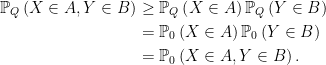
Suppose that X, Y are centered jointly Gaussian random vectors with dimensions m and n respectively, and such that has the covariance matrix . Then, we can write and for some p-dimensional standard Gaussian random vector . Enlarging the probability space if necessary, we can let be another p-dimensional standard Gaussian vector independent from . Setting

the covariance matrix is

Therefore, has the same probability distribution as has under the measure . For symmetric convex sets and ,

Conjecture C1 states that the right hand side of this equality is increasing in t and, hence, conjecture C3 follows. ⬜

---

Royen’s Proof of the Gaussian Correlation Inequality

I now describe Royen’s proof of the Gaussian correlation inequality. The formulation best suited to this approach is inequality (4) above,

(16)

for an n-dimensional centered Gaussian random vector X and any .

The idea behind the proof is then along similar lines to that described in the `local approach’ above. We continuously vary the covariance matrix of X in order to transform the right hand side of (16) into the probability on the left. By differentiating, we aim to show that this gives an increasing function, and (16) will follow.

Laplace transforms will be used to compute the derivatives of the probability as the covariance matrix is varied. Key to this approach is to look at the transforms of the squares, , of the components of X rather than of X itself. The identity

(17)

holds for any nxn positive semidefinite matrix A, where C is the covariance matrix and denotes the determinant. This identity can be computed directly by expressing the expectation in terms of an integral over the Gaussian density.

Defining the random vector Z taking values in by , (17) gives the Laplace transform

(18)

Here, and is the diagonal matrix formed from the components of . To handle the determinant in (18), we will make use of the identity

(19)

The summation is over all finite nonempty subsets J of , denotes the product and is the submatrix of C consisting of the elements with row and column indices in J. So, are the principal minors of C. The first equality in (19) is a classical identity, and follows from expanding out the Leibnitz formula for the determinant of , and the second equality uses the fact that the determinant of is .

Let us now consider the covariance matrix to be a differentiable function of time, . Then, the Laplace transform (18) can be differentiated,

(20)

Now, an important step in Royen’s proof of the Gaussian correlation inequality is to note that the right hand side of (20) can also be expressed in terms of a Laplace transform, but with respect to a different distribution than that used for Z. In fact, is itself a Laplace transform. To show this, for any positive integer d, let be independent centered Gaussian random vectors each with covariance matrix C. Define the n-dimensional random vector . Expressing as the sum of the independent random vectors , each of which has the same distribution as Z above, its Laplace transform can be computed,

(21)

Royen refers to this as an n-variate gamma distribution, which I will denote by . It is just the same thing as the diagonal elements of a matrix with the Wishart distribution, scaled by a factor of 1/2.

Putting the above calculations together, we can now compute how the expectations of functions of Z vary as the covariance matrix C is varied. This is stated in Lemma 3 below. I will deviate slightly from Royen’s argument here. Whereas he expresses the time derivative of the probability density of Z in terms of the probability density, I instead look at the derivatives of the expectation of a smooth function. This avoids some technicalities, such as showing that has smooth probability densities and having to restrict to nonsingular covariance matrices.

Equation (22) below can be compared with (10) above. They both express the derivative of the expectation of a function of our random variables in terms of an expectation over partial derivatives of the function. The difference is that now, we look at expectations of a function of rather than of X directly, and the expectation on the right hand side is with respect to a different probability measure from the original one. Equation (22) does have a more complicated form than (10), involving coefficients which are defined in terms of derivatives of the minors of C. However, these coefficients will be nonnegative in the situation concerning us here, which is all that matters. In the following, I use to denote the mixed partial derivatives

Lemma 3 Let the positive semidefinite matrix be continuously differentiable in parameter t, and X be a centered Gaussian random vector with covariance matrix under the measure , and set . Then, for any smooth with compact support, is continuously differentiable with,

(22)

Here, represents expectation under a probability measure for which has the distribution, and are the coefficients

(23)

Proof: In the case where f is of the form for some fixed , we have and, hence, (22) is given by substituting (21) for into (20) above. The general case then follows by using Laplace or Fourier transform inversion, or by approximating f by linear combinations of functions of the form .

I demonstrate how Fourier transforms allow us to extend to the general case of (22). By analytic continuation, the above can be extended to imaginary values of . So, if we set then (22) will hold with for fixed . If f is smooth of compact support, as in the statement of the lemma, then it can be expressed as

where the Fourier transform is in the Schwartz space of rapidily decreasing functions on . Fubini’s theorem allows us to commute the integral with expectation, and by dominated convergence the partial derivatives commute with the integral, giving

Boundedness and continuity of follows from (20) so, by dominated convergence, we see that is continuously differentiable. ⬜

As in the explanation of the local approach to the correlation conjecture above, we consider covariance matrices which are linearly interpolated between the full covariance matrix of X at and the case at making the first k components of X independent from the final components. Fortunately, in this situation, the coefficients introduced in Lemma 3 are always nonnegative.

Lemma 4 Suppose that covariance matrix is of the form (14),

for rxr matrix , sxs matrix and rxs matrix , with . It is assumed that C is positive semidefinite over . Then, the coefficients defined by (23) are nonnegative.

Proof: For any , can be written as

where are submatrices of respectively. For the moment, suppose that is strictly positive definite, implying that and are positive definite and, in particular, are invertible. Decompose

where is the matrix . Using the block matrix determinant formula,

where runs over the eigenvalues of the positive semidefinite matrix . Then, is decreasing over and, from the assumption that is strictly positive definite, is nonzero. This implies that is nonnegative and decreasing. So, is decreasing in t.

In the case where is not strictly positive definite, the above argument can be applied to the positive definite matrices for any to see that is decreasing in t and, letting go to zero, is decreasing in t, so has nonpositive derivative. Applying this to the definition (23) shows that is nonnegative. ⬜

The previous two lemmas can be combined to show that we can continuously transform the probabilities on the right hand side of inequality (16) into the left hand side in such a way that they are increasing. This is a special case of conjecture C3 above.

Lemma 5 Let X be a random vector with values in and, for each , let be a probability measure with respect to which X is centered Gaussian with covariance matrix of the form (14). Then,

(24)

is increasing in t

Proof: Let Z be the random vector taking values in defined by . Choosing , let be smooth, decreasing, and satisfy for and for . Define by

This is smooth with compact support. For any and we have,

From Lemma 3,

The coefficients are nonnegative, by Lemma 4, so the derivative above is nonnegative and is increasing in t.

Finally, letting go to zero,

so that (24) is increasing in t as claimed. ⬜

Finally, GCI follows from Lemma 5.

Theorem 6 (Gaussian Correlation Inequality) If X is an n-dimensional centered Gaussian random vector then inequality (16),

holds, for each .

Proof: Setting and , write the covariance matrix of X in the form

for rxr matrix , sxs matrix and rxs matrix Q. As this is positive semidefinite, and are positive semidefinite. Letting be defined by (14), is positive semidefinite and, therefore, so is

So, we can define to be a probability measure with respect to which X is centered Gaussian with covariance matrix . Using Lemma 5,

as required. ⬜

---

The Local Method Revisited

Looking at Royen’s proof, it is very similar in appearance to the local method described previously. Both consider continuously varying the coviarance matrix of the joint multidimensional Gaussian random vectors according to (14), and attempt to show that the resulting probabilities are increasing. Royen diverges from previous methods in two ways. First, rather than looking directly at Gaussian measures, by squaring the components of the random vector he instead brings in properties of the multidimensional gamma distribution. Secondly, he considers GCI in the special form (4). This results in showing that the probability (24) stated in Lemma 5 is increasing, rather than the more general form (15) stated in conjecture C3 above.

However, it follows from Royen’s proof that the conjectures discussed in the local approach above are true. It is surprising then that no-one has managed previously to solve the Gaussian correlation inequality using that approach.

Theorem 7 Conjectures C1, C2 and C3 are true.

Proof: We already know, as shown in Lemma 2, that these conjectures are equivalent. I will concentrate on proving C1. That is, if X and Y are independent standard Gaussian random vectors of dimension n then, setting 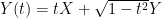, the probability

(25)

is increasing in t over the range . Here, A and B are symmetric convex subsets of .

Consider the case where A and B are convex polytopes of the form (7),

for some and . Defining the (r + s)-dimensional random vector by

its covariance matrix is seen to be as in (14) with , and . By Lemma 5,

is increasing in t.

This proves the result for convex polytopes. As was noted above, every closed symmetric convex set is the limit of a decreasing sequence of convex polytopes. So by taking limits, (25) is increasing in t for any closed symmetric convex sets A and B. Finally, if the sets are symmetric and convex we can use the fact that their closures and have the same Gaussian measures as A and B to conclude that (25) is increasing in t. ⬜

---

References

1. Das Gupta, S., Eaton, M. L., Olkin, I., Perlman, M., Savage, L. J., Sobel, M. (1972)Inequalitites on the probability content of convex regions for elliptically contoured distributions Proceedings of the Sixth Berkeley Symposium on Mathematical Statistics and Probability, Vol. 2: Probability Theory, University of California Press, 241–265. Link
2. Hargé, Gilles (1999) A Particular Case of Correlation Inequality for the Gaussian Measure. The Annals of Probability. Vol. 27, No. 4, 1939–1951. doi:10.1214/aop/1022874822
3. Khatri, C.G. (1967) On Certain Inequalities for Normal Distributions and their Applications to Simultaneous Confidence Bounds. Ann. Math. Statist. 38, No. 6, 1853–1867. doi:10.1214/aoms/1177698618
4. Latała, R., and Matlak, D. (2017) Royen’s Proof of the Gaussian Correlation Inequality. Geometric Aspects of Functional Analysis: Israel Seminar (GAFA) 2014–2016, Springer International Publishing, 265–275. doi:10.1007/978-3-319-45282-1_17. Preprint (2015) available at arXiv:1512.08776
5. Lipton, R.J., Regan, K.W. A Great Solution. Gödel’s Lost Letter and P=NP (blog), 30 Apr 2017.
6. Pitt, Loren D. (1977) A Gaussian Correlation Inequality for Symmetric Convex Sets. The Annals of Probability. Vol. 5, No. 3, 470–474. doi:10.1214/aop/1176995808.
7. Royen, T. (2014) A simple proof of the Gaussian correlation conjecture extended to multivariate gamma distributions. Far East Journal of Theoretical Statistics. Vol 48, Issue 2, 139–145. Preprint available at arXiv:1408.1028
8. Sidak, Z. (1967) Rectangular Confidence Regions for the Means of Multivariate Normal Distributions. Journal of the American Statistical Association. Vol. 62, No. 318, 626–633. doi:10.2307/2283989
9. Sidak, Z. (1968) On Multivariate Normal Probabilities of Rectangles: Their Dependence on Correlations. The Annals of Mathematical Statistics. Vol. 39, No. 5, 1425–1434. Link
10. Retired German man solves one of world’s most complex maths problem with simple proof. Independent, Mon 3 April 2017.
11. Retired 67-year-old man solves one of the world’s most complex maths problems while brushing his teeth using a ‘surprisingly simple’ solution. Daily Mail, Tues 4 April 2017.
12. A Long-Sought Proof, Found and Almost Lost. Quanta Magazine, 28 Mar 2017.