Algebraic Probability: Quantum Theory

We continue the investigation of representing probability spaces as states on algebras. Whereas, previously, I focused attention on the commutative case and on classical probabilities, in the current post I will look at non-commutative quantum probability.

Quantum theory is concerned with computing probabilities of outcomes of measurements of a physical system, as conducted by an observer. The standard approach is to start with a Hilbert space ${\mathcal H}$ , which is used to represent the states of the system. This is a vector space over the complex numbers, together with an inner product ${\langle\cdot,\cdot\rangle}$ . By definition, this is linear in one argument and anti-linear in the other,

$\displaystyle \setlength\arraycolsep{2pt} \begin{array}{rl} &\displaystyle\langle\phi,\lambda\psi+\mu\chi\rangle=\lambda\langle\phi,\psi\rangle+\mu\langle\phi,\chi\rangle,\smallskip\\ &\displaystyle\langle\lambda\phi+\mu\psi,\chi\rangle=\bar\lambda\langle\phi,\chi\rangle+\bar\mu\langle\psi,\chi\rangle,\smallskip\\ &\displaystyle\langle\psi,\phi\rangle=\overline{\langle\phi,\psi\rangle}, \end{array}$

for ${\phi,\psi,\chi\in\mathcal H}$ and ${\lambda,\mu\in{\mathbb C}}$ . Positive definiteness is required, so that ${\langle\psi,\psi\rangle > 0}$ for ${\psi\not=0}$ . I am using the physicists’ convention, where the inner product is linear in the second argument and anti-linear in the first. Furthermore, physicists often use the bra–ket notation ${\langle\phi\vert\psi\rangle}$ , which can be split up into the `bra’ ${\langle\phi\vert}$ and `ket’ ${\vert\psi\rangle}$ considered as elements of the dual space of ${\mathcal H}$ and of ${\mathcal H}$ respectively. For a linear operator ${A\colon\mathcal H\rightarrow\mathcal H}$ , the expression ${\langle\phi,A\psi\rangle}$ is often expressed as ${\langle\phi\vert A\vert\psi\rangle}$ in the physicists’ language. By the Hilbert space definition, ${\mathcal H}$ is complete with respect to the norm ${\lVert\psi\rVert=\sqrt{\langle\psi,\psi\rangle}}$ .

The space of bounded linear operators ${\mathcal H\rightarrow\mathcal H}$ will be denoted by ${B(\mathcal H)}$ , with the adjoint of ${A\in\mathcal H}$ denoted by ${A^*}$ , so that

$\displaystyle \langle\phi,A\psi\rangle=\langle A^*\phi,\psi\rangle.$

This makes ${B(\mathcal H)}$ into a *-algebra. Quantum mechanics involves states, observables, and transformations in the following way. I use ${\mathbb S^1}$ to denote the unit circle ${\{\omega\in{\mathbb C}\colon\lvert\omega\rvert=1\}}$ .

A (pure) state is represented by a vector ${\psi\in\mathcal H}$ normalised so that ${\lVert\psi\rVert=1}$ . Any other vector ${\psi^\prime=\omega\psi}$ with ${\omega\in\mathbb S^1}$ represents the same physical state. If ${\phi,\psi\in\mathcal H}$ are states then, if a system is in pure state ${\psi}$ , the probability of it being in state ${\phi}$ is ${\lvert\langle\phi,\psi\rangle\rvert^2}$ . I will also use non-normalised states in what follows, for which ${\lVert\psi\rVert}$ need not equal 1, with the understanding that it should be normalised to ${\psi/\lVert\psi\rVert}$ before performing calculations.
A measurement may only be able to determine whether the system is in a closed subspace ${V\subseteq\mathcal H}$ . If the system is in state ${\psi}$ , then the probability of being found in the given subspace of states is ${\lVert P_V\psi\rVert^2}$ , where ${P_V}$ represents orthogonal projection onto the subspace. If the measurement is `perfect’, so that it does not interfere with the system in any other way, then a positive measurement result leaves the system in the state ${P_V\psi}$ .
The complete set of possible distinct results of a measurement can be represented by a set of pairwise orthogonal and closed subspaces ${V_n\subseteq\mathcal H}$ such that ${\sum_nV_n}$ is dense in ${\mathcal H}$ . Letting ${P_n}$ represent orthogonal projection onto subspace ${V_n}$ , then orthogonality is equivalent to ${P_mP_n=0}$ for ${m\not=n}$ . Completeness of the set of outcomes is equivalent to ${\sum_nP_n=1}$ . If the system is in pure state ${\psi}$ then, the probability of the measurement giving outcome ${n}$ is ${\lVert P_n\psi\rVert^2}$ , after which it will be in state ${P_n\psi}$ .
Observables are represented by self-adjoint operators. I consider bounded observables, which are represented by operators ${A\in B(\mathcal H)}$ satisfying self-adjointness ${A^*=A}$ . Many of the observables encountered in practice, such as position, momentum, energy, etc., are unbounded. For simplicity, I ignore this fact and will just consider the bounded case. Suppose that an observable ${A\in B(\mathcal H)}$ has a complete set of (normalised) eigenvectors ${e_n\in\mathcal H}$ , with distinct eigenvalues ${a_n}$ . As ${A}$ is self-adjoint, the eigenvalues are real, and the eigenvectors will be orthogonal. A measurement of ${A}$ determines which of the eigenstates ${e_n}$ the system is in, and determines the value of ${A}$ as the associated eigenvalue. If the system starts in state ${\psi}$ , then ${A}$ has probability ${\lvert\langle e_n,\psi\rangle\rvert^2}$ of having value ${a_n}$ . Hence, the expected value is,

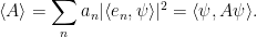$\displaystyle \langle A\rangle=\sum_n a_n\lvert\langle e_n,\psi\rangle\rvert^2=\langle\psi,A\psi\rangle.$ (1)

This can be generalised to the degenerate case where the eigenvalues are not distinct by, instead, considering the orthogonal projections ${P_n}$ onto the eigenspaces, so that ${A=\sum_na_nP_n}$ . Further generalisation to continuous spectra can be achieved using the spectral theorem, although (1) still holds for the expectation.

Note that orthogonal projection onto a closed subspace is a special type of observable which takes only the values 0 and 1, in which case (1) gives the probability of the system being measured to be in the subspace.
Transformations and symmetries of the state space are represented by unitary operators ${U\in B(\mathcal H)}$ . By definition, these satisfy ${U^*U=UU^*=1}$ and take a state ${\psi}$ to the new state ${U\psi}$ . Note that, if ${\omega\in\mathbb S^1}$ , then ${\omega U}$ represents the same transformation as ${U}$ . Examples include space translations, rotations, and time evolution. Continuous transformation groups ${{\mathbb R}\rightarrow B(\mathcal H)}$ , ${t\mapsto U_t}$ , satisfying ${U_sU_t=U_{s+t}}$ are associated with observables by ${U_t=\exp(iAt)}$ . For example, space translations correspond to momentum, rotations correspond to angular momentum, and time evolution corresponds to the total energy of the system. Some discrete transformations, such as time reversal, are represented by anti-unitary operators.
Given two physical systems represented by Hilbert spaces ${\mathcal H_1}$ and ${\mathcal H_2}$ , the composite system is represented by the tensor product ${\mathcal H=\mathcal H_1\otimes\mathcal H_2}$ . An operator ${A}$ on the space ${\mathcal H_1}$ is represented, in the composite system by, by ${A\otimes I}$ . Similarly, an operator ${B}$ on ${\mathcal H_2}$ is represented by ${I\otimes B}$ in the composite system.

Of course, for a full physical model of a system, we would need to relate actual physical measurements to specific observable operators, and describe the time evolution of the system. That is not the aim of this post, however.

The existence of states ${\phi,\psi}$ such that ${\lvert\langle\phi,\psi\rangle\rvert\not\in\{0,1\}}$ means that probabilities are unavoidable in quantum theory. If a system is prepared in the pure state ${\psi}$ , then measured to determine if it is in state ${\phi}$ , an affirmative result occurs with probability ${\lvert\langle\phi,\psi\rangle\rvert^2}$ . The non-squared quantity ${\langle\phi,\psi\rangle}$ is called a probability amplitude. This is not a physically observable quantity, although it is used to explain phenomena such as interference observed in the double-slit experiment, as probability amplitudes can add constructively or cancel due to phase differences.

I also note that, as with classical probability theory, states on quantum systems are subjective. Observers may correctly assign different states to the same system, due to differing levels of knowledge. Whenever a measurement is made, an observer will update their state in accordance with the rules above, whereas a separate observer, who is not aware of the measurement result, will not update their state in the same way.

Mixed States

We can combine classical probability with pure quantum states, to obtain what are known as mixed states. Given a probability measure ${\mu}$ on the set of states ${\psi\in\mathcal H}$ with ${\lVert\psi\rVert=1}$ , we consider the mixture of quantum and classical probability, where ${\mu}$ gives the probability of the physical system being in any measurable set of pure states. If a specific outcome of an experiment on a system in a pure state ${\psi\in\mathcal H}$ occurs with probability ${q(\psi)}$ , then its probability of occurring in the mixed state is ${\int q(\psi)d\mu(\psi)}$ . For a quantum observable ${A\in B(\mathcal H)}$ , its expected value in a pure state is given by (1). Hence, in the mixed state described by ${\mu}$ , its expected value is

$\displaystyle p(A)=\int\langle\psi,A\psi\rangle d\mu(\psi).$

(2)

This expectation operator, ${p\colon B(\mathcal H)\rightarrow{\mathbb C}}$ , is a linear map which is

self-adjoint: ${p(A^*)=\overline{p(A)}}$ .
positive: ${p(A^*A)\ge0}$ .
normalized: ${p(1)=1}$ .

In our language established in the previous post, ${p}$ is a state on the *-algebra ${B(\mathcal H)}$ . A vitally important fact about mixed states is that all physically observable consequences are incorporated in the expectation operator. Any property of the state that cannot be expressed in terms of ${p}$ is not physical. I explain below how the effects of measurements and transformations on a mixed state can be described using the expectation operator alone.

As outlined above, an outcome of a measurement is represented by an orthogonal projection ${P}$ . The probability of the outcome represented by ${P}$ is given, in the mixed state, by ${p(P)}$ . Then, assuming that the measurement is `perfect’, if it gives an affirmative result, the system will be described by a new mixed state ${q}$ given as,

$\displaystyle q(A)=p(PAP)/p(P).$

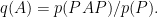(3)

Note that this bears a significant similarity to the formula for classical conditional probabilities. The set of possible distinct results of a measurement is represented by a set of orthogonal projections satisfying ${\sum_nP_n=1}$ . This ensures that ${\sum_np(P_n)=1}$ , which is clearly necessary to interpret ${p(P_n)}$ as probabilities.

Transformations of the system were described above by the action of unitary operators on pure states. However, the action associated to a unitary operator ${U}$ can be expressed just as easily on a mixed state, and takes ${p}$ to a new expectation operator ${q}$ ,

$\displaystyle q(A)=p(U^*AU).$

Anti-unitary operators on the state can also be described simply in terms of their effect on the expectation operator ${p}$ , and are of the form

$\displaystyle q(A)=p(U^*A^*U)$

for anti-unitary ${U\colon\mathcal H\rightarrow\mathcal H}$ .

I now note that certain mixed states with distinctly different descriptions can have the same expectation operator so, in fact, represent the same physical state. Consider a Hilbert space with finite dimension ${d > 1}$ and let ${\phi_1,\ldots,\phi_d}$ and ${\psi_1,\ldots,\psi_d}$ be two orthonormal bases. Also, let ${\mu}$ be the uniform distribution on the space of unit vectors in ${\mathcal H}$ . We have three distinct mixed states, (i) each pure state ${\phi_n}$ occurs with probability ${1/d}$ , (ii) each pure state ${\psi_n}$ occurs with probability ${1/d}$ and, (iii) the distribution of pure states is given by ${\mu}$ . The fact that the trace of a square matrix is independent of the basis chosen shows that these mixed states all have the same expectation operator and, hence, represent equivalent descriptions of the system,

$\displaystyle \setlength\arraycolsep{2pt} \begin{array}{rl} \displaystyle\frac1d\sum_n\langle\phi_n,A\phi_n\rangle &\displaystyle=\frac1d\sum_n\langle\psi_n,A\psi_n\rangle\smallskip\\ &\displaystyle=\int\langle\psi,A\psi\rangle d\mu(\psi)\smallskip\\ &\displaystyle=\frac1d{\rm Tr}(A). \end{array}$

This demonstrates that, once we mix classical probabilities with quantum states, they can never be disentangled. The classical probability distribution is not something that can be observed.

An alternative method of describing mixed states is with trace class operators. For a classical probability measure ${\mu}$ on the space of pure states, we can form the self-adjoint and nonnegative operator,

$\displaystyle \rho=\int\vert\psi\rangle\langle\psi\vert\,d\mu(\psi).$

I am using the physicsts’ bra–ket notation. Alternatively, ${\rho\in B(\mathcal H)}$ maps each vector ${\phi\in\mathcal H}$ to

$\displaystyle \rho\phi=\int\langle\psi,\phi\rangle\psi\,d\mu(\psi).$

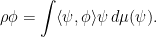
This fully describes the physical state, since the expectation operator (2) can be written as

$\displaystyle p(A)={\rm Tr}(\rho A)={\rm Tr}(A\rho).$

In particular, using ${A=I}$ gives ${{\rm Tr}(\rho)=1}$ . Conversely, any nonnegative ${\rho\in B(\mathcal H)}$ with unit trace describes a mixed state. This is because ${\rho}$ has a complete set of orthonormal eigenvectors ${\psi_n}$ , with corresponding eigenvalues ${p_n\ge0}$ satisfying ${\sum_np_n=1}$ . Then,

$\displaystyle {\rm Tr}(\rho A)=\sum_np_n\langle\psi_n,A\psi_n\rangle,$

so ${\rho}$ represents a system with probability ${p_n}$ of being in the pure state ${\psi_n}$ .

I now consider how mixed states can arise. First, they can occur in the same way that probabilities enter into classical physics — the probability measure ${\mu}$ describes the ignorance that we have regarding the `true’ state of the system. Given a set ${S}$ of pure states of the system, we do not know whether the state of the system in question lies in ${S}$ , so only assign a probability ${\mu(S)}$ . However, there are other ways that mixed states can occur due to the inherently probabilistic nature of quantum theory.

Consider a system in pure state ${\psi}$ , and suppose that we perform a measurement whose possible outcomes are represented by orthogonal projections ${\sum_nP_n=1}$ . A measurement result of `n’ occurs with probability ${\lVert P_n\psi\rVert^2}$ . This outcome leaves the system in the pure state ${P_n\psi}$ . Suppose that we perform the measurement but have not, as yet, observed the result. Then, the system will be in a mixed state, where the pure state ${P_n\psi}$ occurs with probability ${\lVert P_n\psi\rVert^2}$ . More generally, if prior to the measurement, the system is described by an expectation operator ${p}$ then, after the measurement but before observing the result, the system will be described by the new expectation

$\displaystyle q(A)=\sum_np(P_nAP_n).$

(4)

Another method by which mixed states arise, is due to interactions with an external physical system. Suppose that the system is represented with a Hilbert space ${\mathcal H}$ , and the external system is described by ${\mathcal H^\prime}$ . The composite system is represented by the tensor product ${\mathcal H\otimes\mathcal H^\prime}$ . An observable ${A\in B(\mathcal H)}$ is described by ${A\otimes I}$ in the composite system. For a state of the composite system of the form ${\psi\otimes\phi}$ with ${\lVert\psi\rVert=\lVert\phi\rVert=1}$ , the expectation is

$\displaystyle \langle \psi\otimes\phi,(A\otimes I)(\psi\otimes\phi)\rangle=\langle\psi,A\psi\rangle,$

which is just the same as for the pure state ${\psi\in\mathcal H}$ . However, more general pure states for the combined system are of the form ${\chi=\sum_n\psi_n\otimes\phi_n}$ , and it is always possible to choose ${\phi_n}$ to be an orthonormal basis for ${\mathcal H^\prime}$ . Normalisation of the state means that ${\sum_n\lVert\psi_n\rVert^2=1}$ . Then, the expectation is

$\displaystyle \langle\chi,(A\otimes I)\chi\rangle=\sum_n\langle\psi_n,A\psi_n\rangle.$

This describes a mixed state for which the system is in each of the pure states ${\psi_n}$ with probability ${\lVert\psi_n\rVert^2}$ . Any such state, in which more than one of the ${\psi_n}$ is nonzero, is called entangled. Entangled states can arise from non-entangled ones of the form ${\psi\otimes\phi}$ due to unitary evolution in the presence of interactions between the systems. This process, by which pure states evolve to mixed states by interaction with the external environment is described by quantum decoherence.

The Algebra Of Observables

As described above, a quantum system is represented by a Hilbert space ${\mathcal H}$ . A state on this system, whether pure or mixed, is described by a linear map ${p\colon B(\mathcal H)\rightarrow{\mathbb C}}$ which is self-adjoint, positive and normalized so that ${p(1)=1}$ . These properties are expressed using the property of ${B(\mathcal H)}$ as a *-algebra, and does not explicitly require that it is a set of bounded operators on ${\mathcal H}$ . More generally, the observables could generate a strict sub-algebra ${\mathcal A\subseteq B(\mathcal H)}$ , and the state can be regarded as a map ${p\colon\mathcal A\rightarrow{\mathbb C}}$ .

A set of (self-adjoint) observables ${A_1,\ldots,A_n\in\mathcal A}$ are simultaneously measurable if they commute, ${A_iA_j=A_jA_i}$ . In the Hilbert space representation, this means that they can be simultaneously diagonalised (at least, if they have a discrete spectrum). Hence, it is possible in theory to simultaneously measure their values. As we have previously seen, commutativity is also sufficient to imply a uniquely joint probability distribution for ${A_1,\ldots,A_n}$ . That is, there is a unique probability measure ${\mu}$ on ${{\mathbb R}^n}$ satisfying

$\displaystyle p(f(A_1,\ldots,A_n))=\int f(x_1,\ldots,x_n) d\mu(x_1,\ldots,x_n).$

(5)

for all polynomials ${f\in{\mathbb C}[X_1,\ldots,X_n]}$ . On the other hand, if the observables do not commute, then the left hand side of (5) is not even defined, as polynomials can only be evaluated at commuting values of the arguments ${X_1,\ldots,X_n}$ . In fact, there may not even be any probability measure on ${{\mathbb R}^n}$ which is consistent with the distributions of the commuting subsets of ${A_1,\ldots,A_n}$ , as shown by Bell’s inequality.

Any single possible outcome of a measurement on a quantum system is described by an orthogonal projection ${P\colon\mathcal H\rightarrow\mathcal H}$ . This can also be described using the *-algebra properties: an element ${P\in\mathcal A}$ is an orthogonal projection if and only if ${P^*P=P}$ or, equivalently, if ${P}$ is self-adjoint and ${P^2=P}$ . I will denote the collection of orthogonal (or, self-adjoint) projections in ${\mathcal A}$ by ${\mathcal{P(A)}}$ . Two projections, ${P,Q\in\mathcal{P(A)}}$ are mutually orthogonal iff ${PQ=0}$ . Furthermore, we can define a partial order on ${\mathcal{P(A)}}$ by ${P\le Q}$ iff ${PQ=P}$ or, equivalently, if ${Q-P\in\mathcal{P(A)}}$ . Roughly speaking, we can think of projections as akin to events, or measurable sets, in classical probability theory, and ${p(P)}$ is the probability of the event. Two events ${P,Q}$ are simultaneously measurable if they commute, with ${PQ}$ and ${P+Q-PQ}$ representing, respectively, their intersection and union. The complement of an event ${P}$ is ${1-P\in\mathcal{P(A)}}$ , and the inequality ${P\le Q}$ represents containment of ${P}$ in ${Q}$ .

Given two systems represented by Hilbert spaces ${\mathcal H_1}$ and ${\mathcal H_2}$ , the composite system is represented by their tensor product ${\mathcal H=\mathcal H_1\otimes\mathcal H_2}$ . For operators ${A\in B(\mathcal H_1)}$ and ${B\in B(\mathcal H_2)}$ , we form the operator ${A\otimes B}$ on ${\mathcal H}$ by

$\displaystyle (A\otimes B)(\phi\otimes\psi)=(A\phi)\otimes(B\psi).$

More generally, we can form operators in ${B(\mathcal H)}$ by taking finite sums ${\sum_nA_n\otimes B_n}$ of ${A_n\in\mathcal B(\mathcal H_1)}$ and ${B_n\in B(\mathcal H_2)}$ . For finite dimensional Hilbert spaces, all operators in ${B(\mathcal H)}$ can be expressed in this form, so that

$\displaystyle B(\mathcal H)\cong B(\mathcal H_1)\otimes B(\mathcal H_2)$

is the tensor product. More generally, ${B(\mathcal H)}$ will be the closure of the tensor product in the weak (or strong) operator topology. This suggests that, if we represent the two systems by *-algebras ${\mathcal A_1}$ and ${\mathcal A_2}$ , then the composite system is represented by their tensor product ${\mathcal A=\mathcal A_1\otimes\mathcal A_2}$ , or some completion of this. There are natural homomorphisms

$\displaystyle \setlength\arraycolsep{2pt} \begin{array}{rl} &\displaystyle\mathcal A_1\rightarrow\mathcal A,\ a\mapsto a\otimes1,\smallskip\\ &\displaystyle\mathcal A_2\rightarrow\mathcal A,\ b\mapsto 1\otimes b. \end{array}$

The images of any element of ${\mathcal A_1}$ and any element of ${\mathcal A_2}$ commute, showing that ${\mathcal A}$ is a kind of `commutative product’ of the two algebras. Furthermore, for any states ${p_1\colon\mathcal A_1\rightarrow{\mathbb C}}$ and ${p_2\colon\mathcal A_2\rightarrow{\mathbb C}}$ , there is a unique state ${p\colon\mathcal A\rightarrow{\mathbb C}}$ satisfying

$\displaystyle p(a\otimes b)=p_1(a)p_2(b).$

This is a kind of independent product of the states, similar to the product measure in classical probability. Entangled states on ${\mathcal A}$ are precisely those which cannot be expressed in this form.

The use of the tensor product to represent the composite of quantum subsystems does have a very important physical consequence. Suppose that we have two systems represented by *-algebras ${\mathcal A_1}$ and ${\mathcal A_2}$ . I will identify each of these with its image in the *-algebra ${\mathcal A=\mathcal A_1\otimes\mathcal A_2}$ representing the composite system. Suppose, also, that we have a state ${p\colon\mathcal A\rightarrow{\mathbb C}}$ , and two observers, one for each of the two subsystems, and that the second observer makes a measurement on the second system. The possible measurement outcomes are described by a sequence of mutually orthogonal projections ${P_n\in\mathcal P(\mathcal A_2)}$ satisfying ${\sum_nP_n=1}$ . If the outcome is `n’, then this observer updates her state to be ${q(a)=p(P_naP_n)/p(P_n)}$ , in accordance with (3). Now, the two subsystems need not be physically interacting in any way, and could well be at completely different places in the the universe. The first observer may not be in any communication with the second one, or be observing the second subsystem at all. We can compute the impact of the measurement on the state of the first subsystem, as seen by the first observer. This is updated according to (4). Making use of the fact that ${\mathcal A_1}$ and ${\mathcal A_2}$ commute with each other, the updated state for any ${a\in\mathcal A_1}$ is,

$\displaystyle \setlength\arraycolsep{2pt} \begin{array}{rl} \displaystyle q(a) &\displaystyle=\sum_np(P_naP_n)=\sum_np(aP_n^2)\smallskip\\ &\displaystyle=p\left(a\sum_nP_n\right)=p(a). \end{array}$

The measurement has no effect on the first system, which is as it should be. The alternative would inevitably lead to contradictions, or to systems being continually impacted by some spooky action at a distance due to measurements or transformations on other systems with which they may have become entangled at some point in the past.

	Harry on Filtrations and Adapted P…
	Anonymous on Analytic Sets
	Daniel on Analytic Sets
	Sid on Martingale Convergence
	northwiz on Preservation of the Local Mart…
	George Lowther on Martingale Convergence
	Sid on Martingale Convergence
	George Lowther on The Burkholder-Davis-Gundy Ine…
	George Lowther on Preservation of the Local Mart…
	northwiz on Preservation of the Local Mart…

Algebraic Probability: Quantum Theory

Mixed States

The Algebra Of Observables

Published by George Lowther

Leave a Reply Cancel reply

Mixed States

The Algebra Of Observables

Like this:

Related

Published by George Lowther

Leave a Reply Cancel reply