So far, we have been considering positive linear maps on a *-algebra. Taking things a step further, we want to consider positive maps which are normalized so as to correspond to expectations under a probability measure. That is, we require  , although this is only defined for unitial algebras. I use the definitions and notation of the previous post on *-algebras.
Definition 1 A state on a unitial *-algebra  is a positive linear map
  satisfying .
Examples 3 and 4 of the previous post can be extended to give states.
Example 1 Let  be a probability space, and be the bounded measurable maps
  . Then, integration w.r.t.
  defines a state on ,

Example 2 Let  be an inner product space, and be a *-algebra of the space of linear maps
  as in example 2 of the previous post, and including the identity map
  . Then, any
  with
with  defines a state on ,

As I am not considering algebras to be unitial by default, it is desirable to generalise definition 1 to include the non-unitial case. It is always possible to extend a *-algebra to a unitial *-algebra, by taking the direct sum  . This consists of pairs
  for
for  and
and  , which I will denote more simply as
  . The algebra operations are defined as

for  and
and  . It can be seen that this makes into a unitial *-algebra, with unit
  , and can be identified with the sub-*-algebra of elements
  for .
for .
In order to define a state , we will require  to be a positive linear map. We then ask whether can be extended to a state on the unitial *-algebra , satisfying definition 1. Any such extension is uniquely determined by the normalisation condition
  , so that
 |
(1) |
For this to be a state, we just need to show that it is positive.
Lemma 2 Let be a *-algebra and be a positive linear map. Defining
 |
(2) |
then extends to a state on if and only if  .
.
Proof: We extend to by (1), and just need to verify when this is positive. For  ,
,
![\displaystyle \setlength\arraycolsep{2pt} \begin{array}{rl} \displaystyle p\left((\lambda+a)^*(\lambda+a)\right)&\displaystyle=p\left(\bar\lambda\lambda+(\bar\lambda a+\lambda a^*+a^*a)\right)\smallskip\\ &\displaystyle=\lvert\lambda\rvert^2+2\Re[\bar\lambda p(a)]+p(a^*a). \end{array}](https://s0.wp.com/latex.php?latex=%5Cdisplaystyle++%5Csetlength%5Carraycolsep%7B2pt%7D+%5Cbegin%7Barray%7D%7Brl%7D+%5Cdisplaystyle+p%5Cleft%28%28%5Clambda%2Ba%29%5E%2A%28%5Clambda%2Ba%29%5Cright%29%26%5Cdisplaystyle%3Dp%5Cleft%28%5Cbar%5Clambda%5Clambda%2B%28%5Cbar%5Clambda+a%2B%5Clambda+a%5E%2A%2Ba%5E%2Aa%29%5Cright%29%5Csmallskip%5C%5C+%26%5Cdisplaystyle%3D%5Clvert%5Clambda%5Crvert%5E2%2B2%5CRe%5B%5Cbar%5Clambda+p%28a%29%5D%2Bp%28a%5E%2Aa%29.+%5Cend%7Barray%7D+&bg=ffffff&fg=000000&s=0&c=20201002)
By standard properties of quadratics, this is nonnegative for all  iff
iff
By the definition of  , this holds for all iff . ⬜
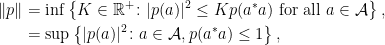
In the case where the algebra is unitial, then the norm  defined by (2) is given simply by
  .
.
Lemma 3 If is a positive linear map on unitial *-algebra then  .
.
Proof: By Cauchy–Schwarz,

with equality when  , giving . ⬜
This suggests the following definition of state on a *-algebra, which is both consistent with the unitial case and ensures that the state can be extended to .
Definition 4 A state on a *-algebra is a positive linear map with  .
.
A *-algebra together with a state reflects the concept of a classical probability space, with representing the algebra of random variables and being the expectation. It also incorporates the extension to quantum probability, by allowing the algebra to be noncommutative. However, it is much too simplistic to serve as a definition of a probability space in keeping with the classical, commutative, theory. In the Kolmogorov axiomatisation, random variables are given by measurable functions, which are closed under various operations, such as taking limits of increasing sequences of variables. We do not simply allow any algebra of functions, such as the polynomials ![{{\mathbb C}[X]}](https://s0.wp.com/latex.php?latex=%7B%7B%5Cmathbb+C%7D%5BX%5D%7D&bg=ffffff&fg=000000&s=0&c=20201002) , to represent the space of all random variables. To simplify the statements in this post, however, I adopt some terminology for a pair
, to represent the space of all random variables. To simplify the statements in this post, however, I adopt some terminology for a pair  consisting of a *-algebra and a state . I use `NC’ as an abbreviation for `noncommutative’, although the algebras in question are not actually required to be noncommutative. We are simply incorporating the noncommutative case in addition to the commutative algebras of classical probability theory.
Definition 5 A *-probability space (or NC preprobability space)[1] is a pair , where is a *-algebra and is a state.
If is a unitial *-algebra and is a (nontrivial) positive linear map, then will be a positive real number. Multiplying by  will give a state. This shows that positive linear maps defined on a unitial *-algebra can be uniquely expressed as a scalar multiple of a state. The situation for non-unitial *-algebras is a bit different. Similar to infinite classical measures, it is possible for to be infinite, in which case cannot be scaled to give a state.
Example 3 Let be the commutative non-unitial *-algebra of complex polynomials ![{f\in{\mathbb C}[X]}](https://s0.wp.com/latex.php?latex=%7Bf%5Cin%7B%5Cmathbb+C%7D%5BX%5D%7D&bg=ffffff&fg=000000&s=0&c=20201002) with zero constant term,
with zero constant term,  .
.
Define so that  is the coefficient of
  in
in  . Then,
  for all
  , so that is positive and
  . Hence, is not a multiple of a state on .
The expectation,  semi-norm, and
  semi-norms, as defined in the previous post, are ordered in the same way as for classical probability spaces.
Lemma 6 If is a *-probability space and then,

Proof: First, by the condition that ,
giving the left hand inequality. Applying the same inequality with  in place of
  ,
,

Cancelling  from both sides gives the right hand inequality. ⬜
In classical probability spaces, it is common to define the  -norm of a random variable by
 ![{\lVert X\rVert_n={\mathbb E}[\lvert X\rvert^n]^{\frac1n}}](https://s0.wp.com/latex.php?latex=%7B%5ClVert+X%5CrVert_n%3D%7B%5Cmathbb+E%7D%5B%5Clvert+X%5Crvert%5En%5D%5E%7B%5Cfrac1n%7D%7D&bg=ffffff&fg=000000&s=0&c=20201002) , where
, where  can be any real number in the range
  . A useful and well-known feature of the norms is that they are increasing in . Looking, now, at *-probability spaces, the random variables are replaced by elements of an algebra . We would like to look at the equivalent norms in this setting, so would be something like
  with the notation of this post. In a general *-algebra, the absolute value
  is not defined. However, for integer , then
  can be written as
  , which is a well-defined element of the algebra.
Lemma 7 Let be a *-probability space. Then, for any , the sequence  is increasing in positive integer .
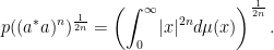
In fact, as was previously noted, for a self-adjoint element of a *-algebra , and state , there exists a probability measure on the real line  such that

for all polynomials . In particular, for any , then is self-adoint, so we can let be its distribution, which will be supported on  . Then,
Hence, lemma 7 can be implied from the classical case. It is good, however, to have a direct proof using *-algebras. In fact, the proof of lemma 7 is a consequence of lemma 8 below.
A sequence  of nonnegative reals, over nonnegative integer , is log-convex if it satisfies

for all  and reals
  with
with  . Equivalently,
  and
and  . In particular, choosing
  and
and  ,
,
 |
(3) |
It can be seen that (3) over the range  is equivalent to log-convexity.
Lemma 8 Let be a *-probability space. For any , define the sequence

for positive integer , and  . Then, is log-convex in
  .
.
Proof: By passing to if necessary, we may suppose that is unitial. Then define a sequence  by
by  and
and

Using  for even , we see that
  , so is self-adjoint. Hence, if m and n are even then
  . Similarly, if m and n are both odd then,

Hence, by Cauchy–Schwarz, for all ,

This is equivalent to log-convexity of , and implies that  is increasing in (exercise!). ⬜
As lemma 7 shows that is increasing in , the limit as goes to infinity will converge to a nonnegative limit (although it could be infinite). This gives an alternative approach to defining an norm on the algebra. In fact, in many cases, it will give the same result as the  semi-norm defined above. Interestingly, Terry Tao uses exactly this definition of the norm in his posts on NC probability, although he does concentrate on tracial states.
A state is called tracial if it satisfies  for all . In particular, if the algebra is commutative, then every state is tracial. Note, however, that the property of being tracial is much weaker than commutativity of the underlying algebra. For example, if is tracial then,

for all  . That is, we can take cyclic permutations without affecting the state. This does not apply for non-cyclic permutations so,
  will generally differ from
  . Straightforward examples of tracial states are given by (multiples of) the trace of an nxn complex matrix.
Lemma 9 Let be a *-probability space and . Then,

Furthermore, if is commutative or, more generally, if is tracial, then we have equality,
Proof: For brevity, I will use  to denote in the proof. Using corollary 6 of the previous post, we have

giving the first inequality. We now assume that the state is tracial, and show that equality is obtained. Choosing any  with
with  , we show that
 |
(4) |
for all nonnegative integer . This follows from induction. The case with  is immediate, from the definition of the norm. Next, suppose that (4) holds for some . Using Cauchy–Schwarz,

we see that (4) also holds for  . So, by induction, (4) holds for all nonnegative integer as claimed. Now, using the fact that is tracial, and applying Cauchy–Schwarz,

Substituting this into (4) gives

Now let go to infinity,

⬜
The previous lemma shows that for tracial states, at least, the semi-norm coincides with  . For non-tracial states, however, this can fail, and can fail quite dramatically.
Example 4 A *-probability space and such that, for all ,

Let be the vector space of measurable and square integrable functions  with compact support (up to almost-everywhere equivalence), and use the inner product

Let ![{\xi=1_{[0,1]}\in V}](https://s0.wp.com/latex.php?latex=%7B%5Cxi%3D1_%7B%5B0%2C1%5D%7D%5Cin+V%7D&bg=ffffff&fg=000000&s=0&c=20201002) , so that . Fixing a measurable and locally bounded
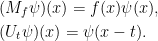
, so that . Fixing a measurable and locally bounded  , we define the `multiplication by ‘ operator
  , and for all
  , define translation by
  ,
,
It can be seen that these have adjoints  and
and  . So, and
  generate a (unitial) *-algebra of linear operators on . Define the state
We now choose to be identically zero on the interval ![{[0,1]}](https://s0.wp.com/latex.php?latex=%7B%5B0%2C1%5D%7D&bg=ffffff&fg=000000&s=0&c=20201002) , so that
, so that  for all . If, in addition, is not essentially bounded on , then
  . We can take
  , and
, and  gives the required example.
It could be argued that the previous example involves unbounded elements of the algebra so, maybe, equivalence of the two norms may hold if the elements are bounded. I will say that a *-probability space is bounded if every is bounded. Even in this case, the equivalence of the two norms can fail in as bad a way as possible.
Example 5 A bounded *-probability space and such that, for all ,

This example follows in the same way as in the previous one except that, here, we choose with essential supremum  . For example,
  . Then, and are bounded operators, so is bounded. As before, and, now,
  .
.
Although I am not requiring algebras to be unitial, *-probability spaces do always contain a sequence approximating a unit in the sense.
Lemma 10 Let be a *-probability space. Then, there exists a sequence  such that
  and
and  .
.
For any such sequence,
-
 is -Cauchy
-
 for all .
-
 for all bounded .
-
 in
in  for all bounded .
- if is unitial then
 , wrt .
- in , wrt .
Proof: By definition (2) of the norm , there exists a sequence with  and
and  . By scaling, we can choose . Then, we can multiply by
  with
with  and
and  , to ensure that
  . So, as required.
Extending the state to , as given by lemma 2,
This shows several things: that  in wrt and, hence, is -Cauchy. If is itself unitial, then it shows that in . Now, for any ,

giving the second point.
Next, suppose that is bounded. Then,

Letting  go to infinity,

Then, let go to infinity to obtain,

giving the third point. Finally, we compute

so that in . ⬜
Suppose that is contained in a larger *-algebra  , and that a state extends to state
  on . We consider how the and semi-norms of these two NC probability spaces compare. I use prime a superscript (
 ) to denote constructions in the larger *-algebra. It is straightforward to show that the semi-norm and inner product agree. For
  ,
,

so that  . On the other hand, the fact that the seminorm involves taking a supremum (equation 3 of the previous post) over the elements of the algebra, means that it can increase when we pass to the larger algebra.

The extreme case is given by example 4, where  in the sub-*-algebra generated by , but
  in the larger *-algebra. When dealing with non-unitial *-algebras, a useful trick is to embed it in the larger, unitial, *-algebra . It is important, then, to know that the norm remains unchanged.
Lemma 11 Let be a *-probability space. Then, for any , its semi-norm is the same computed in as in .
Proof: Let us denote the semi-norm of computed in by  . As is a subalgebra of , we have
  for all , so only the reverse inequality needs to be shown. As it is immediate when
  is infinite, we assume that is bounded. Then, for
  , let be as in lemma 10.

so that  as required. ⬜
In general, if is an element of a *-probability space with zero operator norm, , then we can effectively treat as if it is zero. The collection of all such elements can be characterised in various ways.
Lemma 12 Let be a *-probability space. For , the following are equivalent.
- .
-
 for all .
-
 for all .
If is commutative or, more generally, is tracial, then these are also equivalent to the following,
-
 .
.
-
 for all .
Proof: 1 ⇒ 2: The second statement follows from the inequality,

2 ⇒ 3: The third statement is just a special case of the second.
3 ⇒ 2: Writing  for
for  , the polarization identity gives,

As the third statement says that  , the second statement follows.
2 ⇒ 1: The first statement follows from

We have shown that the first three statements are equivalent. Now, consider the case where is tracial.
4 ⇒ 5: If is tracial, the fifth statement follows from,

5 ⇒ 4: If is tracial, the fourth statement follows from,

with  .
.
5 ⇒ 2: If is tracial then the second statement follows from,
Note that, so far, we have made no use of the fact that is a state. In the case where is unitial, then this is not required at all and, if is non-unitial, it is only needed to show that the last two statements follow from the first three.
2 ⇒ 5: If is a state then the fifth statement follows from,

⬜
It would be useful to have a term to describe a state on a *-algebra for which  whenever . The word faithful would seem to fit, but this is already taken to describe the property that whenever . Except in certain cases, such as for tracial states, this is a much stronger condition than we want. So, instead, I will say that a state for which whenever is nondegenerate or separating, and similarly say that the *-probability space is nondegenerate or separated. This captures the idea that it is equivalent to the topology being separated (i.e., it is T0, T1, or Hausdorff, which are equivalent conditions for a topological vector space).
It is always possible to turn a *-probability space into a nondegenerate one, by quotienting out by the *-ideal of elements satisfying . A subset  of a *-algebra is called a *-ideal if it is a subspace as a complex vector space, and is closed under involution and by multiplication by elements of the algebra. Then, the quotient
  is the collection of equivalence classes
 ![{[a]=\mathcal I+a}](https://s0.wp.com/latex.php?latex=%7B%5Ba%5D%3D%5Cmathcal+I%2Ba%7D&bg=ffffff&fg=000000&s=0&c=20201002) , for . It is made into a *-algebra by,
, for . It is made into a *-algebra by,
![\displaystyle \setlength\arraycolsep{2pt} \begin{array}{rl} &\displaystyle [a]+[b]=[a+b],\smallskip\\ &\displaystyle \lambda[a]=[\lambda a],\smallskip\\ &\displaystyle [a][b]=[ab],\smallskip\\ &\displaystyle [a]^*=[a^*], \end{array}](https://s0.wp.com/latex.php?latex=%5Cdisplaystyle++%5Csetlength%5Carraycolsep%7B2pt%7D+%5Cbegin%7Barray%7D%7Brl%7D+%26%5Cdisplaystyle+%5Ba%5D%2B%5Bb%5D%3D%5Ba%2Bb%5D%2C%5Csmallskip%5C%5C+%26%5Cdisplaystyle+%5Clambda%5Ba%5D%3D%5B%5Clambda+a%5D%2C%5Csmallskip%5C%5C+%26%5Cdisplaystyle+%5Ba%5D%5Bb%5D%3D%5Bab%5D%2C%5Csmallskip%5C%5C+%26%5Cdisplaystyle+%5Ba%5D%5E%2A%3D%5Ba%5E%2A%5D%2C+%5Cend%7Barray%7D+&bg=ffffff&fg=000000&s=0&c=20201002)
and we have the canonical *-homomorphism ![{a\mapsto[a]}](https://s0.wp.com/latex.php?latex=%7Ba%5Cmapsto%5Ba%5D%7D&bg=ffffff&fg=000000&s=0&c=20201002) .
.
Lemma 13 Let be a *-probability space, and  denote the set of with . Then, is a *-ideal, so that the quotient
  is a *-algebra, and
  for all
  .
.
Furthermore, factors uniquely through a nondegenerate state on given by,
![\displaystyle p^\prime([a])=p(a)](https://s0.wp.com/latex.php?latex=%5Cdisplaystyle++p%5E%5Cprime%28%5Ba%5D%29%3Dp%28a%29+&bg=ffffff&fg=000000&s=0&c=20201002)
for all .
Proof: If  ,
,  , and then,

showing that  ,
,  ,
,  and
and  are all in . Hence, is a *-ideal. Next, if and is the sequence given by lemma 10 then,

We just need to show that the extension of to is nondegenerate. However, if ![{\lVert [a]\rVert_\infty^\prime=0}](https://s0.wp.com/latex.php?latex=%7B%5ClVert+%5Ba%5D%5CrVert_%5Cinfty%5E%5Cprime%3D0%7D&bg=ffffff&fg=000000&s=0&c=20201002) then , so that and
then , so that and ![{[a]=0}](https://s0.wp.com/latex.php?latex=%7B%5Ba%5D%3D0%7D&bg=ffffff&fg=000000&s=0&c=20201002) as required. ⬜
as required. ⬜
1 Note: In the initial version of this post, I exclusively used the term `NC preprobability space’. This was updated to use the term `*-probability space’, which is a bit cleaner and more consistent with the terminology of C*-probability and W*-probability spaces to be introduced in a later post, and mirrors the definitions of *-algebras, C*-algebras and W*-algebras.

This is a really interesting post, thank you, I wrote a paper covering definitions of lots of the things described here a while back , http://vixra.org/abs/1203.0011 Best, –Stephen
thanks!
In the quantum group community it is common to use notation that refers to virtual objects. Are you aware of this fashion? It is rather seductive.
I am not entirely sure…I think you might be referring to considering a non-commutative algebra as functions on some underlying space (or group, etc), although this is only really correct if the algebra is commutative. Is that along the correct lines?