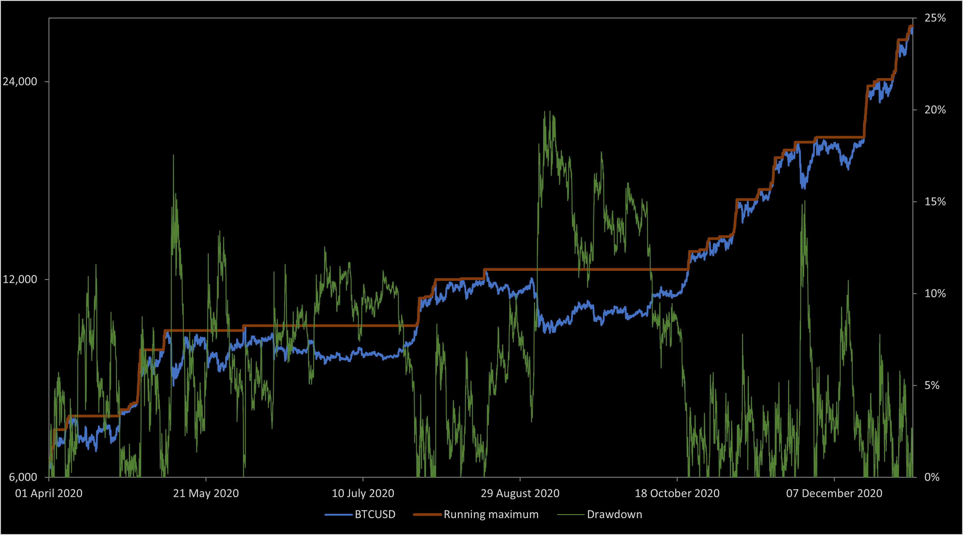
Figure 1: Bitcoin price and drawdown between April and December 2020
For a continuous real-valued stochastic process with running maximum , consider its drawdown. This is just the amount that it has dropped since its maximum so far,
which is a nonnegative process hitting zero whenever the original process visits its running maximum. By looking at each of the individual intervals over which the drawdown is positive, we can break it down into a collection of finite excursions above zero. Furthermore, the running maximum is constant across each of these intervals, so it is natural to index the excursions by this maximum process. By doing so, we obtain a point process. In many cases, it is even a Poisson point process. I look at the drawdown in this post as an example of a point process which is a bit more interesting than the previous example given of the jumps of a cadlag process. By piecing the drawdown excursions back together, it is possible to reconstruct from the point process. At least, this can be done so long as the original process does not monotonically increase over any nontrivial intervals, so that there are no intervals with zero drawdown. As the point process indexes the drawdown by the running maximum, we can also reconstruct X as . The drawdown point process therefore gives an alternative description of our original process.
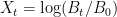
See figure 1 for the drawdown of the bitcoin price valued in US dollars between April and December 2020. As it makes more sense for this example, the drawdown is shown as a percent of the running maximum, rather than in dollars. This is equivalent to the approach taken in this post applied to the logarithm of the price return over the period, so that . It can be noted that, as the price was mostly increasing, the drawdown consists of a relatively large number of small excursions. If, on the other hand, it had declined, then it would have been dominated by a single large drawdown excursion covering most of the time period.
For simplicity, I will suppose that and that tends to infinity as t goes to infinity. Then, for each , define the random time at which the process first hits level ,
By construction, this is finite, increasing, and left-continuous in . Consider, also, the right limits . Each of the excursions on which the drawdown is positive is equal to one of the intervals . The excursion is defined as a continuous stochastic process equal to the drawdown starting at time and stopped at time ,
This is a continuous nonnegative real-valued process, which starts at zero and is equal to zero at all times after . Note that there uncountably many values for but, the associated excursion will be identically zero other than for the countably many times at which . We will only be interested in these nonzero excursions.
As usual, we work with respect to an underlying probability space , so that we have one path of the stochastic process X defined for each . Associated to this is the collection of drawdown excursions indexed by the running maximum.
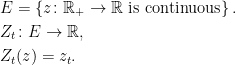
As S is defined for each given sample path, it depends on the choice of , so is a countable random set. The sample paths of the excursions lie in the space of continuous functions , which I denote by E. For each time , I use to denote the value of the path sampled at time t,
Use to denote the sigma-algebra on E generated by the collection of maps , so that is the measurable space in which the excursion paths lie. It can be seen that is the Borel sigma-algebra generated by the open subsets of E, with respect to the topology of compact convergence. That is, the topology of uniform convergence on finite time intervals. As this is a complete separable metric space, it makes into a standard Borel space.
Lemma 1 The set S defines a simple point process on ,
for all .
From the definition of point processes, this simply means that is a measurable random variable for each and that there exists a sequence covering E such that are almost surely finite. The set of drawdowns for the point process corresponding to the bitcoin prices in figure 1 are shown in figure 2 below.
Figure 2: Bitcoin price drawdowns between April and December 2020


on
,
.