Probability Space Extensions and Relative Products

According to Kolmogorov’s axioms, to define a probability space we start with a set Ω and an event space consisting of a sigma-algebra F  on Ω. A probability measure ℙ on this gives the probability space (Ω, F , ℙ), on which we can define random variables as measurable maps from Ω to the reals or other measurable space.

However, it is common practice to suppress explicit mention of the underlying sample space Ω. The values of a random variable X: Ω → ℝ are simply written as X, rather than X(ω) for ω ∈ Ω. It is intuitively thought of as a real number which happens to be random, rather than a function. For one thing, we usually do not really care what the sample space is and, instead, only care about events and their probabilities, and about random variables and their expectations. This philosophy has some benefits. Frequently, when performing constructions, it can be useful to introduce new supplementary random variables to work with. It may be necessary to enlarge the sample space and add new events to the sigma-algebra to accommodate these. If the underlying space is not set in stone then this is straightforward to do, and we can continue to work with these new variables as if they were always there from the start.

Definition 1 An extension π of a probability space (Ω, F , ℙ) to a new space (Ω′, F ′, ℙ′),

is a probability preserving measurable map π: Ω′ → Ω. That is, ℙ′(π^-1E) = ℙ(E) for events E ∈ F .

By construction, events E ∈ F  pull back to events π^-1E ∈ F ′ with the same probabilities. Random variables X defined on (Ω, F , ℙ) lift to variables π^∗X with the same distribution defined on (Ω′, F ′, ℙ′), given by π^∗X(ω) ≡ X(π(ω)). I will use the notation X^∗ in place of π^∗X for brevity although, in applications, it is common to reuse the same symbol X and simply note that we are now working with respect to an enlarged the probability space if necessary.

The extension can be thought of in two steps. First, the enlargement of the sample space, π: Ω′ → Ω on which we induce the sigma algebra π^∗F  consisting of events π^-1E for E ∈ F , and the measure ℙ′(π^-1E) = ℙ(E). This is essentially a no-op, since events and random variables on the initial space are in one-to-one correspondence with those on the enlarged space (at least, up to zero probability events). Next, we enlarge the sigma-algebra to F ′ ⊇ π^∗F  and extend the measure ℙ′ to this. It is this second step which introduces new events and random variables.

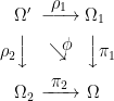
Since we may want to extend a probability space more than a single time, I look at how these combine. Consider an extension π of the original probability space, and then a further extension ρ of this.

These can be combined into a single extension ϕ = π○ρ of the original space,

Lemma 2 The composition ϕ = π○ρ is itself an extension of the probability space.

Proof: As compositions of measurable maps are measurable, it is sufficient to check that ϕ preserves probabilities. This is straightforward,

for all E ∈ F . ⬜

So far, so simple. The main purpose of this post, however, is to look at the situation with two separate extensions of the same underlying space. Both of these will add in some additional source of randomness, and we would like to combine them into a single extension.

Separate probability spaces can be combined by the product measure, which is the measure on the product space for which the projections onto the original spaces preserves probability, and for which the sigma-algebras generated by these projections are independent. Recall that a pair of sigma-algebras F  and G  defined on a probability space are independent if, for any sets A ∈ F  and B ∈ G  then ℙ(A ∩ B) = ℙ(A)ℙ(B).

Combining extensions of probability spaces will, instead, make use of relative independence.

Definition 3 Let (Ω, F , ℙ) be a probability space. Two sub-sigma-algebras G , H  ⊆ F  are relatively independent over a third sigma-algebra K  ⊆ G  ∩ H  if

(1)

for all A ∈ G  and B ∈ H .

It can be shown that the following properties are each equivalent to this definition;

• 𝔼[XY|K ] = 𝔼[X|K ]𝔼[Y|K ] for all bounded G -measurable random variables X and H -measurable Y.
• 𝔼[X|G ] = 𝔼[X|K ] for all bounded H -measurable X.
• 𝔼[X|H ] = 𝔼[X|K ] for all bounded G -measurable X.

Once a probability measure is specified separately on G  and H  then its extension to the sigma-algebra generated by G  ∪ H , if it exists, is uniquely determined by relative independence. This is a consequence of the pi-system lemma, since (1) defines it on the events {A ∩ B: A ∈ G , B ∈ H }, which is a pi-system generating the same sigma-algebra.

Now consider two separate extensions π₁ and π₂ of the same underlying probability space,

As maps between sets, these can both be embedded into a single extension known as the pullback or fiber product. This is the set Ω′= Ω₁ ×_Ω Ω₂ defined by

Defining projection maps ρ_i: Ω′ → Ω_i by

results in a commutative square with ϕ ≡ π₁○ρ₁ = π₂○ρ₂,

In fact, Ω′ is exactly the cartesian product Ω₁ × Ω₂ restricted to the subset on which π₁○ρ₁ and π₂○ρ₂ agree.

This constructs an extension ϕ of the sample space containing π₁ and π₂ as sub-extensions. However, it still needs to be made into a probability space. Use the smallest sigma-algebra F ′ on Ω′ making ρ₁, ρ₂ into measurable maps, which is generated by ρ₁^∗F ¹ ∪ ρ₂^∗F ². The probability measure ℙ′ on (Ω′, F ′) is uniquely determined on each of the sub-sigma-algebras by the requirement that ρ_i preserve probabilities,

for i = 1, 2 and A ∈ F ⁱ. These necessarily agree on ϕ^∗F  ⊆ ρ₁^∗F ¹ ∩ ρ₂^∗F ²,

for A ∈ F . The natural way to extend ℙ′ to all of F ′ is to use relative independence over ϕ^∗F .

Definition 4 The relative product of the extensions π₁ and π₂ is the extension

with ϕ, Ω′, F ′ constructed as above, and ℙ′ is the unique probability measure for which the projections ρ₁, ρ₂ preserve probabilities, and for which ρ₁^∗F ¹ and ρ₂^∗F ² are relatively independent over ϕ^∗F .

The measure ℙ′ is also known as the relative product measure. As noted previously, relative independence is enough to uniquely determine the extension of ℙ′ from the ρ_i^∗F ⁱ sub-sigma-algebras. So, the relative product measure is uniquely determined, if it exists. It is not, however, guaranteed to exist. In almost all cases of interest it will exist, such as for standard Borel spaces and, even if it doesn’t, it still exists as near as makes no difference. I will look at this existence in a moment. For now, assuming that the relative product exists, it gives an extension of probability spaces containing π₁ and π₂ as sub-extensions. This can be expressed as a commutative square,

The ideas outlined above extend to relative products of arbitrarily many extensions but, for simplicity, I concentrate on the product of a pair of extensions.

---

Regular Extensions

One method of extending a probability space (Ω, F , ℙ) uses a transition probability P from (Ω, F ) to a measurable space (Ω′, F ′). This is a map

such that, for each ω ∈ Ω, A ↦ P(ω, A) is a probability measure and, for each A ∈ F ′, ω ↦ P(ω, A) is F -measurable. This induces a probability measure ℙ′ on (Ω′, F ′)

Then a measurable map π: Ω′ → Ω will preserve probabilities and, so, define an extension of probability spaces as long as the transition probability satisfies the condition: for any A ∈ F ′ and ω ∈ Ω ∖ π(A) then P(ω, A) = 0.

Definition 5 An extension of probability spaces

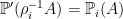
will be called regular if there exists a transition probability P from (Ω, F ) to (Ω′, F ′) such that

for all S ∈ F ′ and P(ω, S) = 0 for all ω ∈ Ω ∖ π(S).

This terminology is specific to this blog and not standard, as far as I am aware. The term ‘regular’ is used since it refers to the existence of regular conditional probabilities for the sub-sigma-algebra F ^∗. So, for A ∈ F ′, the conditional probability can be expressed as

for almost all ω ∈ Ω′. The relevance, for our purposes, is that they guarantee the existence of relative products.

Lemma 6 Let π₁ and π₂ be extensions of probability space (Ω, F , ℙ). If at least one of these is regular, then their relative product exists.

If both π₁ and π₂ are regular then so is their relative product.

Proof: Use the notation above for the relative product (Ω′, F ′, ℙ′). Suppose that π₁ is regular given by a transition probability P₁. For S ∈ F ′, define its probability under measure ℙ′ by,

(2)

There are a few points to consider when interpreting (2). First off, the integral must be restricted to elements (ω₁, ω₂) in Ω′. That is, π₁(ω₁) = π₂(ω₂). Use Ω_1,ω ⊆ Ω₁ to denote the slice of ω₁ ∈ Ω₁ satisfying π₁(ω₁) = ω and F _ω¹ to represent the sigma-algebra F ¹ restricted to this. The integral over ω₁ in (2) is thus restricted to the slice Ω_1,π2(ω2) and, so, the transition probability has to be defined on such slices. This is easy enough, since any element of F _ω¹ is equal to Ω_1,ω ∩ A for some A ∈ F ¹. We set,

This is well-defined since, for any other set B ∈ F ¹ with Ω_2,ω ∩ B = Ω_2,ω ∩ A, then π₁(B ∖ A) and π₁(A ∖ B) both do not contain ω and, so P₁(ω, A) and P₁(ω, B) are equal by assumption.

Next, for (2) to be well-defined, we need 1_{{(ω1,ω2)∈S}} to be F ¹_π2(ω2) measurable with respect to ω₁, and for

to be F ² measurable with respect to ω₂. This parallels the considerations required in proofs of Fubini’s theorem. Trying S = A ×_Ω B for A ∈ F ¹ and B ∈ F ² then 1_{{(ω1,ω2)∈S}} = 1_{ω1∈A}1_{ω2∈B}, which is measurable with respect to ω₁ as required. Integrating,

This is F ² measurable with respect to ω₂ and, by the monotone class theorem, extends to all S ∈ F ′. So, (2) defines a measure ℙ′.

Again using S = A ×_Ω B in (2),

(3)

Putting B = Ω₂ gives,

and A = Ω₁ gives,

so that ρ₁ and ρ₂ preserve probabilities as required. It remains to prove relative independence so, from (3) and using the fact that ρ₂ preserves probabilities,

showing that ρ₁^∗F ¹ and ρ₂^∗F ² are independent conditioned on ϕ^∗F  as required.

Finally, suppose that π₂ is also regular given by the transition probability P₂. Then, (2) gives,

so that ϕ is a regular extension given by the transition probability

⬜

Often, extensions of probability spaces are constructed using a transition probability from the original space to an auxiliary measurable space (X, X ). Some authors use this as the definition of an extension, rather than the considerably more general definition 1 that I use above. While it can seem a bit confusing why they feel the need to introduce such a transition probability, which is unnecessary for many purposes, it does ensure that relative products exist or, in our terminology, that the extension is regular.

Lemma 7 Let (Ω, F , ℙ) be a probability space and P be a transition probability from (Ω, F ) to measurable space (X, X ). Setting

then the projection map, π: Ω′ → Ω given by π(ω, x) = ω defines a regular probability space extension.

Proof: This is clearly a valid extension since π preserves probabilities. For any A ∈ F  then (ω, x) is in π^-1A if and only if ω is in A,

Define a transition probability Q from (Ω, F ) to (Ω′, F ′) by

This represents a process going from state ω ∈ Ω to state (ω, x) in the product Ω × X, where x is randomly distributed according to P(ω, ·) and ω stays fixed. Integrating,

as required by definition 5. The only remaining point is that, if ω ∈ Ω ∖ π(S) then (ω, x) ∉ S for all x ∈ X and so,

⬜

Regular conditional probabilities are guaranteed to exist for random variables taking values in standard Borel spaces. These are measurable spaces constructed as the Borel sigma-algebra associated with a Polish space. That is, (Y, Y ) is standard Borel if there exists a complete separable metric on the sample space Y for which Y  is the sigma algebra generated by open sets. The great thing about standard Borel spaces is that they are both general enough for many purposes but, also, very special in other ways. They are quite general in that measurable subspaces, countable products, and countable disjoint unions all preserve the standard Borel property. The real numbers with the usual Borel sigma-algebra is standard. It follows that any countable collection {ξ_i}_i∈I of real random variables can be represented as a single variable taking values in standard Borel space ℝ^I. This extends to countable collections of real-valued stochastic processes in continuous time which are continuous, cadlag, or right continuous. This is because they can be represented by their values at rational times. On the other hand, every standard Borel space is either countable or isomorphic (as a measurable space) to the real numbers with its usual Borel sigma-algebra.

The following is a standard result for the existence of regular conditional probabilities, but I include a proof here for completeness.

Lemma 8 Let (Ω, F , ℙ) be a probability space and ρ, ξ be random variables taking values in measurable spaces (X, X ) and (Y, Y ) respectively.

If Y is a standard Borel space then there exists a transition probability P from X to Y satisfying

almost surely, for all A ∈ Y .

Proof: As Y is standard Borel, it can be assumed to be a closed subset of ℝ with the Borel sigma-algebra. For all q ∈ ℚ define the conditional cumulative distribution function of ξ as

for almost all x ∈ X. For rational numbers q, r, the following are satisfied for almost all x ∈ X,

• F_x(q) ≤ F_x(r) whenever q < r.
• F_x(q) = F_x(r) whenever q < r and (q, r] is disjoint from Y.
• F_x(q) → 1 as q → ∞.
• F_x(q) → 0 as q → -∞.

As these are countably many constraints, they will all be simultaneously satisfied outside of a zero probability event. Replacing F_x with whatever we like on this null event, we can suppose that the above conditions are satisfied for all x. Now, set

This will satisfy all the conditions above for all real q, r. As it is also right-continuous in y it defines a transition probability from X to Y by

for all A ∈ Y . Choosing A = (-∞, y] gives

By the monotone class lemma this holds for all A ∈ Y . ⬜

Consider an extension of probability spaces

and ξ: Ω′ → X be a random variable taking values in a measurable space (X, X ). Then, π can be restricted to a subextension ρ formed by just adding this random variable to the original space.

(4)

Here, ρ(ω, x) = ω is the projection onto Ω and ℚ(A) = ℙ′((π × ξ)^-1A) is the induced probability measure on F  ⊗ X . By construction, ρ preserves probabilities so is an extension of probability spaces. Also, the joint distribution of π and ξ in the initial extension has the same joint distribution as ρ and the projection ξ′(ω, x) = x do in the new one. Hence, if ξ incorporates all the additional randomness required in our extension, then we may as well use the extension ρ instead.

Corollary 9 In (4), if (X, X ) is a standard Borel space then the extension ρ is regular.

Proof: Using lemma 8 there exists a transition probability P from (Ω, F ) to (X, X ) satisfying

for all A ∈ E  and almost all ω ∈ Ω. So, for all A ∈ F  and B ∈ X  we obtain

By the monotone class lemma this holds for A × B replaced by any element of F  ⊗ X . So lemma 7 says that ρ is a regular extension. ⬜

---

Example – Extensions for which there is no relative product

Above, I showed that with rather mild constraints, relative products of probability spaces exist. However, I did not show that they exist in general. This is because they don’t! So, to gain an idea of how it can go wrong, I give an example of two extensions of a probability space for which there is no relative product. This example may seem a bit unnatural, which is to be expected, since in most practical cases the product does exist.

Let us start with the uniform measure on the unit interval. So Ω = [0, 1), F  is the Lebesgue sigma-algebra, and ℙ is the Lebesgue measure on Ω. Next, for our example, we will need a subset A of Ω with zero inner measure and unit outer measure. That is, every measurable subset of A has zero measure and every measurable superset in Ω has measure 1. This is necessarily non-measurable. Examples do exist, such as Vitali sets. The idea is that our probability space contains a random variable X uniformly distributed on the unit interval. We construct an extension containing a random variable X_A ∈ A such that X_A = X almost surely, and a separate extension containing a variable X_B ∈ Ω ∖ A such that X_B = X almost surely. These cannot both exist in the same extension since, then, X_A = X = X_B almost surely, which is impossible since they lie in disjoint sets.

Now define a space (A, F _A, ℙ_A), where elements of F _A can, by definition, be written as A ∩ E for some E ∈ F , and set ℙ_A(A ∩ E) = ℙ(E). This is well-defined, since if there is another F ∈ F  with the same intersection then the difference of E and F is disjoint from A so has zero measure by assumption, and ℙ(E) = ℙ(F). Defining π_A: A → Ω to be the identity π_A(ω) = ω we have an extension,

Next, set B = Ω ∖ A and construct (B, F _B, ℙ_B) and π_B in exactly the same way as above, but with B in place of A. This gives two extensions of our original probability space.

The fiber product A ×_Ω B is equal to the pairs (a, b) ∈ A × B with a = b. By construction, though, this is empty! Clearly, we cannot define a probability measure on an empty set, so no relative product exists.

The example above might not look very satisfying. Our ‘extensions’ were not really making the probability space bigger. By restricting to the subsets A and B they were actually removing values from the sample space! As they only removed values from a set with zero inner measure, it did not affect the event space (up to zero probability events) or space of random variables but, still, the sample space was smaller. It was for this reason that the fiber product was empty. Maybe we should modify our definition of extensions to require them to be onto? This still does not work, as a simple modification of the above example shows.

With (A, F _A, ℙ_A) as above, let us construct a new space (Ω_A, G _A, ℚ_A) as follows. Take Ω_A to be the product Ω × A and G _A = F  ⊗ F _A to be the product sigma-algebra. Also, letting Δ_A: A → Ω_A be the diagonal map Δ_A(a) = (a, a), we define the probability measure

So, defining π_A: Ω_A → Ω to be the projection π_A(ω, a) = ω this gives an extension

Now π_A is onto. Constructing another extension π_B in the same way using the set B = Ω ∖ A in place of A, we have two extensions of the original probability space. The fiber product is Ω′= Ω × Ω_A × Ω_B together with projections ρ_A: Ω′ → Ω_A and ρ_B: Ω′ → Ω_B given by ρ_A(ω, a, b) = (ω, a) and ρ_B(ω, a, b) = (ω, b).

There is no extension of the measures induced on ρ^∗_AG _A and π^∗_BG _B to all of the sigma-algebra F ′ generated by these. This is for the reason outlined above, the random variables X(ω, a, b) = ω, X_A(ω, a, b) = a and X_B(ω, a, b) = b satisfy X_A = X = X_B almost surely, yet they lie in disjoint sets.

To be precise, consider any measurable set E ∈ F . Then,

up to zero probability events. The left hand equality is using the measure on ρ^∗_AG _A induced by ρ_A and the second us using the measure on ρ^∗_BG _B induced by ρ_B. So, it holds under any extension ℙ′ of these measures to F ′ and, taking intersections,

up to a zero probability event. So, for positive integer n, setting E_k = [2^–n(k - 1), 2^–nk) we have

up to a zero probability event. So, the left hand side has ℙ′ measure equal to 1, but decreases to the diagonal (ω, a, b) with a = b as n → ∞, which is empty. So, the ‘measure’ ℙ′ does not satisfy countable additivity, and the relative product is not defined.

---

Notes

This post has delved a bit deeper into aspects of probability space extensions than is done in many texts on probability theory. For one thing, I look at extensions defined by an arbitrary measure preserving map, whereas some texts only consider extensions defined by a transition probability to an auxiliary space. Lemma 7 above provides one explanation for why some people may prefer to restrict to such special kinds of extension. In my terminology here, they are regular and ensure the existence of relative products. If. however, we were to only consider such types of extensions from the outset then it would be a bit unsatisfactory. As well as seeming a bit artificial requiring an apparently unnecessary transition probability, it would not be clear why this restriction is in place without considering what can go wrong otherwise. The definition of relative products used here follows, loosely, that used by Fremlin, Measure Theory, Chapter 45.

In practice, on the occasion that a particular construction requires extending the probability space, this can be done explicitly as required — usually by taking the independent product with a separate space.

One area where relative products are almost unavoidable is in weak solutions to stochastic differential equations (SDEs). In this case, solutions exist in an extension and, by taking their relative product, we obtain two distinct solutions on the same probability space. If the SDE satisfies pathwise uniqueness, then this would be impossible unless both weak solutions are actually measurable with respect to the original probability space and are equal. That is, they are strong solutions.

Comparing with the literature, Rogers & Williams (Diffusions, Markov Processes, and Martingales: Volume 2, Theorem 17.1) directly makes use of the fact that regular conditional probabilities exist for Polish spaces, and constructs the relative product within the proof for weak solutions of SDEs, without explicitly defining the concept. Kallenberg instead uses the idea of ‘transfer’ of random variables from one probability space to another (Foundations of Modern Probability, 2nd Ed, Theorem 6.10), which is effectively the same thing as a relative product.

As it is an intuitive concept which very simply explains why results such as ‘pathwise uniqueness implies solutions are strong’, I prefer to separate out the idea of relative products here and look at them in their own right.