Non-Measurable Sets

Probability and measure theory relies on the concept of measurable sets. On the real numbers ℝ, in particular, there are several different sigma-algebras which are commonly used, and a set is said to be measurable if it lies in the one under consideration. Probabilities and measures are only defined for events lying in a specific sigma-algebra, so it is essential to know if sets are measurable. Fortunately, most simply constructed events will indeed be measurable, but this is not always the case. In fact, once we start working with more complex setups, such as continuous-time stochastic processes observed at random times, non-measurable sets occur more commonly than might be expected. To avoid such issues, it is usual to enlarge the underlying sigma-algebra defining a probability space as much as possible.

The Borel sets form the smallest sigma-algebra containing the open sets or, equivalently, containing all intervals. This is denoted as , which I will also shorten to . An explicit construction of a non-Borel set was given by Lusin in 1927. Every irrational real number can be expressed uniquely as a continued fraction

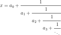where a₀ is an integer and a_i are positive integers for i ≥ 1. Lusin considered the set of irrationals whose continued fraction coefficients contain a subsequence a_k1, a_k2, … such that each term is a divisor of the subsequent term.

Other examples can be given along similar lines to Lusin’s. Every real number has a binary expansion

where a₀ is an integer and a_i is in {0, 1} for each i ≥ 1. Consider the set of reals having a binary expansion for which there is an infinite sequence of positive integers k₁, k₂, …, each term strictly dividing the next, such that a_ki = 1. I will give proofs that these examples are non-Borel in this post.

There is a general method of enlarging sigma-algebras known as the completion. Consider a measure μ defined on a measurable space consisting of sigma-algebra on set X. The completion consists of all subsets S ⊆ X which can be sandwiched between sets in whose difference has zero measure. That is, A ⊆ S ⊆ B for with μ(B ∖ A) = 0. It can be shown that is a sigma-algebra containing , and μ uniquely extends to a measure on this by taking μ(S) = μ(A) = μ(B) for S, A, B as above.

The Lebesgue measure λ is uniquely defined on the Borel sets by specifiying its value on intervals as λ((a, b)) = b – a. The completion is the Lebesgue sigma-algebra, which I will denote by . Usually, when saying that a subset of the reals is measurable without further qualification, it is understood to mean that it is in . The non-Borel set constructed by Lusin can be shown to be measurable (in fact, its complement has zero Lebesgue measure).

While the Lebesgue measure extends uniquely to , this is not true for for all measures defined on the Borel sigma-algebra. In particular, it will not be true for singular measures, which assign a positive value to some Lebesgue-null sets. An example is the uniform probability measure (or, Haar measure) on the Cantor middle-thirds set C. This has zero Lebesgue measure, so every subset of C is in , but the uniform measure on C cannot be extended uniquely to all subsets. For this reason, universal completions are often used. For a measurable space , the universal completion consists of the subsets of X which lie in the completion of with respect to every possible sigma-finite measure.

The intersection is taken over all sigma-finite measures μ on . It is enough to take the intersection over finite or, even, probability measures, since every sigma-finite measure is equivalent to such. The universal completion is a bit tricky to understand in an explicit way but, by construction, all sigma-finite measures on a sigma-algebra extend uniquely to its universal completion. It can be shown that Lusin’s example of a non-Borel set does lie in the universal completion .

Finally, the power set consisting of all subsets of a set X is a sigma-algebra. For uncountable sets such as the reals, this is often too large to be of use and measures cannot be extended in any unique way. However, we have four common sigma-algebras of the real numbers,

(1)

In this post, I show that each of these inclusions is strict. That is, there are subsets of the reals which are not Lebesgue measurable, there are Lebesgue sets which are not in the universal completion , and there are sets in which are not Borel. Lusin’s construction is an example of the latter. The strictness of the other two inclusions does depend crucially on the axiom of choice so, unlike Lusin’s set, the examples demonstrating that these are strict are not explicit.

---

Vitali Sets

Vitali sets are a common example of non-measurable sets. We can define an equivalence relation x ∼ y on the real numbers which holds whenever x – y is rational. This partitions ℝ into a collection of equivalence classes, which consist of sets of the form ℚ + x, equal to all numbers differing from x by a rational number. A Vitali set S is any set containing a single element of each equivalence class. That is, every real number x differs from exactly one element of S by a rational amount. This is not an explicit construction, since it requires the axiom of choice to select a unique element of each equivalence class but, as we will see, this is by necessity.

For each rational number q, let S_q consist of the elements of S + q taken modulo 1. That is, each element x ∈ S is mapped to the unique y ∈ [0, 1) such that x + q – y is an integer. If S was Lebesgue measurable, then S_q would also be Lebesgue, which we can see by writing

For any distinct pair of rational numbers q, r ∈ [0, 1), the sets S_q and S_r are disjoint. For any element x of their intersection, both x – q + m and x – r + n would lie in S for integer m, n, which is not possible as they are distinct elements of the same equivalence class. Also, for any x ∈ [0, 1), the equivalence class ℚ + x contains an element of S and, so, x – q ∈ S for some rational q, giving x ∈ S_q. Hence,

and, if S was Lebesgue measurable, countable additivity gives

(2)

For any pair of rationals q, r, the set S_r is just S_q + r – q modulo 1. By translation invariance of the Lebesgue measure λ(S_q) = λ(S_r) if these are measurable. This contradicts (2). If λ(S_q) was positive, then it gives an infinite sum of equal positive terms, which is infinite. If λ(S_q) was zero, then the sum is zero. In either case, the sum is not 1 so (2) cannot hold. Hence, λ(S_q) is undefined and S is not Lebesgue measurable.

We have constructed subsets of ℝ which are not Lebesgue measurable, so the final inclusion of (1) is strict. Any example S of a non-Lebesgue set is easily modified to give an example of a Lebesgue set which is not in the universal completion of the Borel sigma-algebra. All we need is to find a one-to-one Borel-measurable function f: ℝ → ℝ whose image has zero Lebesgue measure, then f(S) gives the example.

As f(S) is contained in a Lebesgue-null set, it is Lebesgue measurable. To show that it is not in we need to find a sigma-finite measure μ such that it is not in the completion . For this, let λ′ be any finite measure equivalent to λ and take μ = f^∗λ′ defined by

If f(S) was in then there would be Borel sets A ⊆ f(S) ⊆ B with μ(B ∖ A) = 0. Then, f^-1A ⊆ S ⊆ f^-1B and λ′(f^-1B ∖ f^-1A) = 0, showing that S is Lebesgue measurable,a contradiction. Hence, f(S) is Lebesgue measurable but not in .

It just remains to find a one-to-one measurable function f: ℝ → ℝ whose image is Lebesgue-null. An example is the map which takes the binary expansion of a real number and re-interprets it as a decimal expansion. That is, every real number x has a unique binary expansion

for integer a₀ and a_i ∈ {0, 1} for i ≥ 1, which does not terminate with repeating 1’s. This last constraint is required to ensure that the binary expansion is unique. Then,

This is clearly one-to-one and, since Lebesgue almost-every real number contains decimal digits other than 0 and 1 (in fact, they are normal), the image of f is Lebesgue-null. For any Vitali set S, f(S) is an example of a Lebesgue set which is not in , showing that the second inclusion of (1) is strict.

---

The Solovay Model and Axiom of Choice

I constructed sets above which are not Lebesgue measurable, and sets which are Lebesgue but not universally Borel measurable. These constructions based on Vitali sets made essential use of the Axiom of Choice. You may wonder if this is necessarily the case. The answer is yes, as shown by the Solovay model. This is a model of Zermelo-Fraenkel (ZF) set theory in which the axiom of choice does not hold, although dependent choice does, which is sufficient for almost all measure and probability theory.

The important property of the Solovay model for us is that every subset of the real numbers is Lebesgue measurable. This is a very strong statement indeed! If we were to always work within the axiomatic framework of this model of set theory, many technical difficulties encountered in measure theory magically vanish. In fact, it has been proposed that this should be used as the standard framework, especially for measure theory.

So, under the Solovay model, the right hand inclusion in (1) would no longer be strict. Vitali sets simply wouldn’t exist. We can go further though, and show that all subsets being Lebesgue actually implies that they are in .

Consider any atomless probability measure μ on the Borel sigma-algebra, so that μ({x}) = 0 for all points x. Define its cumulative distribution function

which is continuous and increasing from 0 to 1. Then μ(F^-1A) = λ(A) for all Borel A ⊆ [0, 1]. Also, let U ⊆ ℝ be the union of the intervals on which F is constant, which is Borel with zero μ-measure. Any subset A of the reals satisfies F^-1F(A) ∖ U ⊆ A ⊆ F^-1F(A).

For any subset S ⊆ ℝ, F(S) is Lebesgue by assumption, so there exists Borel sets A ⊆ F(S) ⊆ B with λ(B ∖ A) = 0. Then A′= F^-1A ∖ U and B′= F^-1B are Borel with A′ ⊆ S ⊆ B′ and μ(B′ ∖ A′) = 0. Hence, S is in the completion .

Next, if μ is any finite measure on the Borel sigma algebra, let A ⊆ ℝ be its set of atoms, x ∈ ℝ with μ({x}) > 0, which is countable. Its restriction ν to ℝ ∖ A is atomless and, by the above, all subsets of ℝ are in . However, adding a countable set of atoms does not change the completion, so contains all subsets of ℝ. As this holds for all finite measures μ, the universal completion contains all subsets of the reals.

Under the Solovay model, we see that , so the strictness of the second and third inclusions of (1) depends crucially on uncountable choice.

Non-Borel sets can be constructed without appealing to uncountable choice by, instead, using a ‘diagonalization’ argument. The idea is that is generated by a countable collection of subsets of ℝ, such as the open intervals with rational endpoints. Every set can be built from this collection by repeated applications of countable set operations. This construction can be encoded as a Borel code. The number of Borel codes has cardinality of the continuum, so the same is true of . Hence it is possible to index Borel sets as . Then, the set

cannot be Borel. If it was, it would equal B_x for some x ∈ ℝ, giving the contradiction: x ∈ B_x iff x ∉ B_x.

Creating non-Borel sets in this way, without uncountable choice, demonstrates that the inequality is strict, even in the Solovay model. However, the construction is a bit messy and, in ZFC set theory, it is not clear whether it necessarily results in a universally measurable set. Also, it does not tell us about simple explicit examples such as Lusin’s set described at the top of the post. I will make use of analytic sets, represented as projections of closed sets. This allows a similar diagonalization argument to be used and are guaranteed to be universally measurable. Furthermore, analytic sets can be mapped to Lusin’s set, amongst other straightforward examples, proving that they are non-Borel.

---

Analytic Sets

One method of constructing non-Borel sets which are universally measurable is via the theory of analytic sets developed by Lusin. Before detailing such a construction, I go over some of theory first. Just the minimal amount required for our purposes.

Use ℕ = {1, 2, …} to denote the natural numbers (excluding zero, which will be convenient here) and N = ℕ^ℕ for Baire space consisting of infinite sequences of natural numbers. This can be given the product topology, so that a sequence a_n ∈ N  converges to a limit b if, for each k, the k‘th terms (a_n)_k are eventually equal to b_k. This is homeomorphic to the space of irrational numbers in the unit interval (0, 1) with the standard topology by continued fractions,

It can be seen that N  is a Polish space — that is, separable and completely metrizable. Specifically, the set of sequences which eventually terminate in repeating 1’s is countable and dense, showing that it is separable, and a complete metric can be defined by

While there are many different ways of defining analytic subsets of a Polish space, the following will be useful here. For the cartesian product X × Y of sets, I use π: X × Y → X to denote the projection (x, y) ↦ x.

Definition 1 A subset A of Polish space X is analytic if it is equal to π(S) for some closed subset S of X × N .

It can immediately be seen that Lusin’s set described at the top of this post is analytic. Let X ⊆ ℝ be the irrational numbers and S ⊆ X × N  be the pairs (x, c) such that (c₁, c₂, …) is strictly increasing and such that the continued fraction coefficients a₀, a₁, … are such that each a_cn divides a_cn+1. This is closed and π(S) is Lusin’s set which, therefore, is analytic.

A first property of analytic sets is that they are closed under countable unions and intersections.

Lemma 2 The collection of analytic subets of a Polish space X is closed under countable unions and under countable intersections.

Proof: If A₁, A₂, … is a sequence of analytic sets, then there exists a sequence S₁, S₂, … of closed subsets of X × N  such that A_n = π(S_n).

Consider S ⊆ X × N  consisting of pairs (x, a) where a = (n, b₁, b₂, …) for some n ∈ ℕ and (x, b) ∈ S_n. This is closed and x ∈ π(S) iff there exists n ∈ ℕ and b ∈ S_n such that (x, b) ∈ S_n. Equivalently, x ∈ π(S_n) = A_n. So,

is analytic.

Next, let θ: ℕ × ℕ → ℕ be a bijection. Then define S ⊆ X × N  to consist of pairs (x, b) such that the sequence a₁, a₂, … ∈ N  given by (a_n)_m = b_θ(m,n) satisfies (x, a_n) ∈ S_n for all n ∈ ℕ. This is closed and x ∈ π(S) iff there exists a sequence a₁, a₂, … ∈ N  such that (x, a_n) ∈ S_n for all n ∈ ℕ. Equivalently, x ∈ π(S_n) = A_n. So,

is analytic as required. ⬜

An immediate consequence is that all Borel sets are analytic.

Theorem 3 Every Borel subset of a Polish space X is analytic.

Proof: Using A  for the analytic subsets of X, lemma 2 says that it is closed under countable unions and countable intersections. Also, every closed A ⊆ X is equal to π(A × N ) and, so, is in A . Furthermore, as it is a metric space, every open set is the union of an increasing sequence of closed sets. Specifically, if A is closed and, for each n we let B_n consist of the x ∈ X satisfying d(x, y) ≥ 1/n for all y ∈ A, then B_n is an sequence of closed sets increasing to X ∖ A. So, by the monotone class theorem, A  contains the sigma-algebra generated by the closed sets, which are the Borel sets. ⬜

In the other direction, all analytic sets are in the universal completion of the Borel sigma-algebra.

Theorem 4 Every analytic subset of a Polish space X is in the universal completion of the Borel sigma-algebra.

For the proof of this, I refer to other posts of this blog. See, for example, theorem 10 of the post on Choquet’s capacitability theorem, or theorem 5 of the post on measurable projection. These both give proofs that π(S) is universally measurable for any measurable S ⊆ X × ℝ. As we noted above that N  is homeomorphic to (0, 1) ∖ ℚ, these also apply to measurable subsets of X × N  and, in particular, to any closed subset S of X × N .

Using A (X) for the analytic sets, theorems 3 and 4 are summarized by the inclusions

---

Non-Borel Analytic Sets

Having completed the very brief introduction to analytic sets, I will now show how non-Borel examples can be constructed. We start with universal closed sets. Here, for a subset S ⊆ X × Y and y ∈ Y, I use S_y to denote the slice consisting of x ∈ X with (x, y) ∈ S.

Definition 5 For Polish spaces X, Y, a closed subset S ⊆ X × Y will be said to be universal if every closed subset of X is equal to S_y for some y ∈ Y.

We can construct universal closed sets.

Lemma 6 For any Polish space X, there exists a universal closed subset of X × N .

Proof: As X is a separable metrizable space, its topology has a countable basis U₁, U₂, …. For example, the balls of radius 1/n centered at points of a countable dense subset gives a countable basis. I assume that the empty set is also included in the basis, so that every open subset of X is a non-empty union of the U_n.

Now let V ⊆ X × N  consist of pairs (x, a) where x ∈ ⋃_nU_an. This is open and, as every open subset W ⊆ X can be written as a union

we have W = V_a. So, (X × N ) ∖ V is universal closed. ⬜

We now construct a non-Borel set as promised, which uses a diagonalization argument.

Lemma 7 Let S ⊆ N  × N  × N  be universal closed and S′ ⊆ N  × N  consist of the pairs (x, y) such that (x, y, x) ∈ S.

Then, S′ is closed and A = π(S′) is an analytic subset of N  whose complement N  ∖ A is not analytic. In particular, A is not Borel.

Proof: By assumption, every closed subset of N  × N  is equal to S_x for some x ∈ N  and, hence, every analytic subset of N  can be written as π(S_x). If we define B ⊆ N  to be the set of x ∈ N  such that x ∉ π(S_x) then this cannot be analytic. If it was, it would equal π(S_x) for some x but, then, x ∈ B iff x ∉ π(S_x) is a contradiction.

The complement A = N  ∖ B of the non-analytic set just constructed is given by x ∈ A iff x ∈ π(S_x). This is equivalent to (x, y) ∈ S_x for some y, or, (x, y, x) ∈ S. This is the same as (x, y) ∈ S′ , or x ∈ π(S′). So, A = π(S′) has non-analytic complement B. As B is not analytic, theorem 3 says that it is also non-Borel. ⬜

We have constructed a subset of A ⊆ N which is not Borel but, as it is analytic, is in the universal completion of the Borel sigma-algebra. Also, as was noted above, N  is homeomorphic to (0, 1) ∖ ℚ and, hence, we also obtain a subset of the reals which is not Borel but is in the universal completion.

This is enough to prove the claim near the top of the post that the inequality is strict. However, it is not a very expicit example and certainly is not expressed as simply as Lusin’s example. As we will see though, this result can be built on to give a proof that Lusin’s set is not Borel.

---

Lusin’s Non-Borel Set

Lemma 7 above proved the existence of universally measurable sets which are not Borel, so the first inclusion of (1) is strict. Although it was not very explicit, I will show how it can be used to imply that the examples given at the top of this post are also non-Borel.

First, a bit of notation which will be useful. Use ℕⁿ for the length-n sequences of natural numbers and, fo a ∈ N , use a|_n ∈ ℕⁿ for the truncated length-n sequence (a₁, …, a_n). Also, for m ≤ n and a ∈ ℕⁿ, use a|_m ∈ ℕ^m for the turncated length-m sequence (a₁, …, a_m). The disjoint union of finite sequences is countable, and partially ordered by the relation a ≺ b for a ∈ ℕ^m and b ∈ ℕⁿ with m < n and a = b|_m.

The following lemma expresses analytic sets in terms of infinite increasing sequences in N^∗ and has some of the flavour of Lusin’s set.

Lemma 8 Let S be a closed subset of N  × N . For each a ∈ ℕⁿ, let H_a be the set of x ∈ N  such that (x|_n, a) = (y|_n, z|_n) for some (y, z) ∈ S.

Then, the indicator function 1_Ha: N  → {0, 1} is continuous, and x ∈ N  is in π(S) if and only if there is a sequence a_n ∈ N^∗ with a_n ≺ a_n+1 and x ∈ H_an for each n.

Proof: As membership x ∈ H_a is a function of finitely many terms of x (depending only on x|_n, it is continuous or, equivalently, H_a is both open and closed.

Now suppose that x ∈ π(S). Then, (x, y) ∈ S for some y and the trivial identity (x|_n, y|_n) = (x|_n, y|_n) implies, from the definition, that x ∈ H_y|n. However, a_n = y|_n is an increasing sequence for the partial order on ℕ^∗ as required.

Conversely, suppose that there is an increasing sequence a_n with the stated properties. Using k_n for the length of a_n, the fact that it is increasing gives a b ∈ N  with b|_kn = a_n for each n. Also, by assumption there exists (y_n, z_n) ∈ S with y_n|_kn = x|_kn and z_n|_kn = b|_kn for each n. This implies that (y_n, z_n) tends to (x, b) so, as it is closed, is contained in S. Hence, x ∈ π(S) as required. ⬜

Lemma 8 refers to increasing sequences in the partially ordered set N^∗. This can be transferred to increasing sequences in ℕ with the division order (each term divides the next).

Consider Cantor space C = 2^ℕ which is the space of sequences (a₁, a₂, …) in {0, 1} with the product topology. This is a compact Polish space, using the same metric as defined above for Baire space and has the countable dense subset of sequences containing finitely many 1’s. In fact C  can be identified with the closed subspace of N  of sequences whose terms are all 1 or 2.

Let L_C be the subset of Cantor space consisting of x ∈ C  such that there is a sequence k₁, k₂, … of positive integers, each term strictly dividing the next, satisfying x_ki = 1 for each i. This is analytic, since it equals π(S) where S ⊆ C  × N  is the closed set consisting of pairs (x, y) where each term of y strictly divides the subsequent one and x_yi = 1 for each i.

Lemma 9 Every analytic subset of N  is equal to f^-1(L_C) for a continuous map f: N  → C 

Proof: The first thing is to construct a one-to-one map θ: ℕ^∗ → ℕ which is an order isomorphism onto its image, using the division order on ℕ^∗. That is, θ(a) divides θ(b) iff a ≺ b. This can be done by prime factorization. Let p_ij be distinct primes indexed by i, j ∈ ℕ. Then, for a ∈ ℕⁿ, write

If a ≺ b then θ(b) consists of multiplying the same primes as b, as well as some additional ones as b is longer, so θ(a) strictly divides θ(b). Conversely, suppose that θ(a) divides θ(b). If b ∈ ℕⁿ then θ(b) is a product of n distinct primes. As θ(a) divides it, it must be a product of a subset of these primes which, because the p_ij are distinct, can only happen if a ⪯ b.

Now, consider analytic A = π(S) for closed S ⊆ N  × N . Then, let H_a ⊆ N  be as constructed in Lemma 8. We define f: N  → C  as follows. Set f(x) = y = (y₁, y₂, …) where y_θ(a) = 1_{x∈Ha} and y_n = 0 for n not in the image of θ, y_n = 0.

Suppose that x ∈ A. By lemma 8, there is a strictly increasing sequence a_n ∈ ℕ^∗ with x ∈ H_an. Hence, θ(a_n) strictly divides θ(a_n+1) and y_θ(an) = 1 for each n. So, y ∈ L_C.

Conversely, suppose that y ∈ L_C. By definition, there is a sequence n_k of positive integers each strictly dividing the next with y_nk = 1. So, n_k = θ(a_k) for some a_k ∈ ℕ^∗, each a_k ≺ a_k+1a_k+1 and x ∈ H_ak. By lemma 8, this gives x ∈ A as required. ⬜

Let L_N be the subset of Baire space consisting of x ∈ N  such that there is a strictly increasing sequence k₁, k₂, … of positive integers, such that x_ki divides x_ki+1 for each i. This is analytic since L_N = π(S) where S is the closed subset of N  × N  consisting of pairs (x, y) where the terms of y are strictly increasing and x_yi divides x_yi+1.

Lemma 10 There exists a continuous map f: C  → N  such that L_C = f^-1(L_N).

Proof: Starting with a sequence of district prime numbers P = {p₁, p₂, …}, define a one-to-one function θ: ℕ → ℕ to have image in the set of numbers whose prime factors are in P , and which preserves divisibility. That is, m divides n iff θ(m) divides θ(n). This can be done by listing all prime numbers in order, l₁, l₂, …. Then map number with prime factorization l₁^r_n⋯l_n^r_n to p₁^r₁⋯p_n^r_n.

We can choose that the collection P  of prime number to leave out an infinite set of primes q₁, q₂, …, where all q_i are distinct. Then, define f: C  → N  by f(x) = y where y_n = n whenever n = θ(m) for some m with x_m = 1, else set y_n = q_n.

As each y_n only depends on the value of one term of x, f is continuous. Suppose that x ∈ L_C, so that there is a sequence k₁, k₂, … with each term strictly dividing the next and x_ki = 1. So, each n_i = θ(k_i) is a strictly increasing sequence with each term dividing the next and, hence, y_ni = n_i divides y_ni+1, showing that y ∈ L_N.

Conversely, suppose that y ∈ L_N, so that there is a strictly increasing sequence k₁, k₂, … with y_ki dividing y_ki+1. We cannot have y_ki = q_ki since no other terms in y are a multiple of this prime. Hence, k_i = θ(n_i) for some sequence of distinct integers n_i with x_ni = 1. Also, as k_i divides k_i+1, n_i divides n_i+1 and, so, x ∈ L_C as claimed. ⬜

Use L to denote Lusin’s set of irrational numbers whose continued fraction coefficients have a subsequence a_k1, a_k2, … with each term dividing the next. This is analytic in the same way as for L_N as was already noted above.

Finally, use K to denote the real numbers having a binary expansion a₀.a₁a₂⋯ for which there exists a sequence k₁, k₂, … with each term strictly dividing the next and for which a_ki = 1. This can also be seen to be analytic in a similar way as above. Let S be the subset of ℝ × N  consisting of pairs (x, y) where each term in y divides the subsequent one and x has a binary expansion with coefficients satisfying a_yi = 1 for all i. This is closed and K = π(S).

Putting together the results above shows that the sets under consideration are not Borel measurable.

Corollary 11 The sets L_C, L_N, L, K are analytic and, hence, universally measurable, but are not Borel measurable.

Proof: We have already shown that each of these are are analytic and, so, by theorem 4 are universally measurable.

By lemma 7, we can choose analytic and non-Borel A ⊆ N . Then, by lemma 9, A = f^-1(L_C) for some continuous function f: N  → C . So L_C cannot be Borel otherwise A would also be Borel.

Likewise, lemma 10 says that there is a continuous function f: C  → N  with L_C = f^-1(L_N) and, so L_N is not Borel.

Defining the continuous map f: N  → ℝ taking a ∈ N  to the irrational number with continued fraction coefficients 0, a₁, a₂, … is continuous, and L_N = f^-1(L), so L is not Borel.

Define continuous map f: C  → ℝ taking a ∈ C  to the real number with binary expansion 0.a₁a₂…. Then, L_C = f^-1(K) ∖ B, where B is the elements of C  with finitely many 1’s. We need to subtract out the elements with finitely many 1’s, since these map to a number with two binary expansions, one of which ends in repeated 1’s, so is in K. As B is countable, it is Borel and, hence, if K was Borel then L_C would also be Borel which has already been shown to be false. ⬜

The proof that Lusin’s set is not Borel given above is loosely based on the 1978 paper Proof of a theorem of Lusin by V.G. Kanovei