For these initial posts of this blog, I will look at one of the most fascinating objects in mathematics, the Riemann zeta function. This is defined by the infinite sum
 |
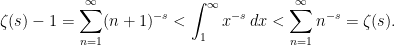
(1) |
which can be shown to be uniformly convergent for all  with
with  . It was Bernhard Riemann who showed that it can be analytically continued to the entire complex plane with a single pole at
  , derived a functional equation, and showed how its zeros are closely linked to the distribution of the prime numbers. Riemann’s seminal 1859 paper is still an excellent introduction to this subject, an English translation of which (On the Number of Prime Numbers less than a Given Quantity) can be found on the Clay Mathematics Institute website, who included the conjecture that the `non-trivial’ zeros all lie on the line
  among their million dollar millenium problems.
In this post I will give a brief introduction to the zeta function and look at its functional equation. In particular, the functional equation can be generalized and reinterpreted as an identity of Mellin transforms, which links the additive Fourier transform on  with the multiplicative Mellin transform on the nonzero reals
  . The aim is to the prove the generalized functional equation and some properties of the zeta function, working from first principles, and discuss at a high level how this relates to the ideas in Tate’s thesis. Some standard complex analysis and Fourier transform theory will be used, but no prior understanding of the Riemann zeta function is assumed.
The zeta function has a long history, going back to the Basel problem which was posed by Pietro Mengoli in 1644. This asked for the exact value of the sum of the reciprocals of the square numbers or, equivalently, the value of  . This was eventually solved by Leonard Euler in 1734 who discovered the famous identity
Euler found the values of  at all positive even numbers, although I will not be concerned with this here. More pertinent to the current discussion is the product expression also found by Euler,
 |
(2) |
The product is taken over all prime numbers  , and converges on . Proving (2) is straightforward. The formula for summing a geometric series gives
Substituting this into (2) and expanding the product gives an infinite sum over terms of the form
for  , primes
  , and integers
  . Using the fact that every positive integer has a unique expression as a product of powers of distinct primes, we see that the Euler product expands as a sum of terms of the form
  as
as  ranges over the positive integers. This is just the right hand side of (1) and shows that the Euler product converges and is equal to
  whenever the sum (1) is absolutely convergent.
The Euler product provides a link between the zeta function and the prime numbers, with far-reaching consequences. For example, the prime number theorem describing the asymptotic distribution of the prime numbers was originally proved using the Euler product, and the strongest known error terms available for this theorem still rely on the link between the prime numbers and the zeta function given by (2). Euler used the fact that (1) diverges at to argue that (2) also diverges at . From this, it is immediately deduced that there are infinitely many primes and, more specifically, the reciprocals of the primes sum to infinity.
The Euler product can also be expressed in terms of the logarithm of the zeta function. Using the Taylor series expansion of  , we obtain
 |
(3) |
As the terms on the right hand side are bounded by  as runs through the subset of the natural numbers consisting of prime powers, it will be absolutely convergent whenever (1) is. In particular, (3) converges on the half-plane . Although the complex logarithm is generally only defined up to integer multiples of
  , (3) gives the unique continuous version of
  over which takes real values on the real line.
We will first look at the zeta functional equation as described by Riemann. This involves the gamma function defined on  by the absolutely convergent integral
 |
(4) |
This is easily evaluated at to get  , and an integration by parts gives the functional equation of
  ,
,
This can be used to evaluate the gamma function at the positive integers,  . Also, by expressing
  in terms of
  , it allows us to extend to a meromorphic function on
  with a single simple pole at
  . Repeatedly applying this idea extends as a meromorphic function on the entire complex plane with a simple pole at each non-positive integer. Furthermore, it is known that is non-zero everywhere on
  .
.
The functional equation can now be stated as follows.
Theorem 1 (Riemann) The function defined by (1) uniquely extends to a meromorphic function on with a single simple pole at of residue  . Setting
 |
(5) |
this satisfies the identity
 |
(6) |
Riemann actually gave two independent proofs of this, the first using contour integration and the second using an identity of Jacobi. Many alternative proofs have been discovered since, with Titchmarsh listing seven (The Theory of the Riemann Zeta Function, 1986, second edition). I will not replicate these here, but will show an alternative formulation as an identity of Mellin transforms, from which Riemann’s functional equation (6) follows as a special case.
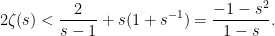
As an example of the use of the functional equation to derive properties of the zeta function on the left half-plane  , we evaluate
  . Using the special value
  and the fact that has a pole of residue at , we see that
  as
as  approaches . Similarly, using the fact that the gamma function has a pole of residue at , we see that
  as approaches
  . Putting these limits into the functional equation gives
Similarly, the functional equation expresses the values of at negative odd integers in terms of its values at positive even integers. For example, taking  ,
,
Plugging in the values  , and Euler’s value of
  ,
,
Via a process known as zeta function regularization, these special values of are sometimes written as the famous, but rather confusing, expressions
Next, using standard properties of the gamma function, theorem 1 can be used to investigate the zeros of the zeta function. The Euler product implies that has no zeros on , as I will show below, and it is well known that the gamma function has no zeros at all. So,  has no zeros or poles anywhere on , and the functional equation extends this statement to
  . It follows that, on , the zeros of the zeta function must cancel with the poles of
  , which are at the negative even integers.
On the strip  , the precise location of the zeros of are not known. However, as has no poles or zeros on this domain (other than at ), they must coincide with the zeros of . From the definition (1) of the zeta function, it satisfies
  (using a bar to denote complex conjugation). So, its zeros are preserved by reflection
  about the real line. Also, by the functional equation, they are preserved by the map
  in the aforementioned strip. We have arrived at the following.
Lemma 2 The function has zeros at the (strictly) negative even integers. The only remaining zeros lie in the vertical strip and are preserved by the maps
 |
(7) |
The zeros at the negative even integers are called the trivial zeros of , with the remaining ones referred to as the non-trivial zeros. The domain is known as the critical strip. So, the non-trivial zeros of the Riemann zeta function are precisely those lying in the critical strip, and are the same as the zeros of the function defined by (5). The vertical line  lying along the center of the critical strip is called the critical line. Then, (7) says that the non-trivial Riemann zeta zeros are symmetric under reflection about both the real line and the critical line. The Riemann hypothesis, as originally conjectured by Riemann in his 1859 paper, states that the non-trivial zeros all lie on the critical line. This, however, remains unknown and is one of the great open problems of mathematics.
We will now move on to the alternative interpretation of the functional equation relating additive Fourier transforms with multiplicative transforms. We will use the following convention for the Fourier transform of a function  ,
,
For this to make sense, it should at least be required that  is integrable. I will restrict to the particularly nice class of Schwartz functions. These are the infinitely differentiable functions from to which vanish faster than polynomially at infinity, along with their derivatives to all orders. That is,
  as
as  , for all integers
  . Denote the space of Schwartz functions by
  . Schwartz functions are integrable and it is known that their Fourier transforms are again in
  . Then, for any
  , its Fourier transform is inverted by
I’ll explain now why the Fourier transform (8) is an additive transform of . For each fixed  , the map
  is a continuous homomorphism from the additive group of real numbers to the multiplicative group of nonzero complex numbers
  ,
,
So, is a character of the reals under addition. Furthermore, integration is invariant under additive translation,
That is, the standard (Riemann or Lesbesgue) integral is the Haar measure of the additive group of reals, and the Fourier transform (8) is the integral of  against additive characters with respect to the additive Haar measure.
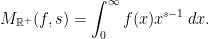
The Mellin transform of is
which is defined for any for which the integral is absolutely convergent. (This differs slightly from the usual definition where a lower limit of is used for the integral. See the note on Mellin transforms at the end of this post.) Now, the map  is a continuous homomorphism from the multiplicative group of nonzero reals to ,
Denoting  , integration with respect to
  is invariant under multiplicative rescaling by any
  ,
,
That is,  is the multiplicative Haar measure on , and the Mellin transform is the integral of against multiplicative characters with respect to the multiplicative Haar measure. This explains why the Fourier transform (8) is additive and the Mellin transform (9) is multiplicative.
For an explicit example of a Mellin transform, consider  ,
,
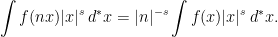
Here, the substitution  was used. Comparing with the definition (4) of the gamma function,
 |
(10) |
For Schwartz functions, the integral defining the Mellin transform is absolutely convergent on the right half-plane , and can be analytically continued to the entire complex plane.
Theorem 3 If  , then
  is well defined over , and uniquely extends to a meromorphic function on with only simple poles at the non-positive even numbers
  , with residue
I’ll give a proof of theorem 3 below. For now, we will move straight on to the statement of the functional equation relating the Mellin transform of to that of its Fourier transform  .
.
Theorem 4 If then  extends to a meromorphic function with only simple poles at and of residue
  and
and  respectively. The functional equation
 |
(11) |
holds everywhere.
A proof of this will be given further down. It can be shown that the specific case is equal to its own Fourier transform,  . So, using expression (10) for the Mellin transform , we see that Riemann’s functional equation follows directly from (11).
Above, we discussed how Riemann’s functional equation allows values of to be determined on the left half-plane and restricts the locations of its zeros to be as described in lemma 2. This made use of properties of the gamma function, specifically the locations of its poles and the fact that it has no zeros. These arguments can be made by instead using version (11) of the functional equation, and the gamma function need not be referred to at all. For an arbitrary smooth function , theorem 3 gives the poles of . Also, by choosing with compact support in , will be well-defined everywhere by (9) and is analytic. It is also easy to choose such that the Mellin transform does not vanish at any specified point, which is enough to apply the arguments above.
I now briefly consider the relation between the functional equation in the form (11) and the ideas of John Tate’s 1950 thesis. Theorem 4 can be viewed primarily as relating the Mellin transform of the Fourier transform to the Mellin transform of the original function. The zeta function plays more of an ancillary role as a multiplicative factor in this identity. This treatment of the Mellin transform as the primary object of interest was taken much further in Tate’s thesis. Tate refocussed attention from the rational and real number fields (or algebraic number field) to the larger ring of adeles,  . This is outside of the scope of this post, but the important properties are that, just like the embedding of the rationals inside the reals,
  embeds in , and the theory of Fourier and Mellin transforms extends to functions defined on the adeles. In the adelic case, he obtained the functional equation
 |
(12) |
Now, the zeta function does not appear at all! Digging a bit deeper, the ring of adeles over the rational numbers can be expressed as a product of the reals and the ring of `finite’ adeles,
That is, every element  of the adelic ring can be expressed as a pair
  consisting of a real number
  and a finite adele
  . For a function
  which is a product of the real and finite parts,
  , the Mellin and Fourier transforms are also products of the transforms of the individual components.
Applying this to the adelic functional equation (12),
Just as the special case  lead to the gamma factor in Riemann’s functional equation, choosing a particular example for the function
  on the finite adeles which equals its own Fourier transform leads to the appearance of the zeta function in (5) and (11). This places the gamma term and the zeta term in the functional equation on a roughly equal footing.
We can go further. The finite adeles can be broken down into a restricted product of fields corresponding to each prime number — the -adic numbers,
In the case where the function  factors into a product of functions on the -adic components,
  , then the Mellin transform commutes with this factorisation,
For a particular choice of , specifically the indicator function of the integral adeles, this is just the Euler product described above. From this viewpoint, the gamma factor in Riemann’s functional equation, the Mellin transform appearing in (11), the Riemann zeta function, and the  terms in the Euler product, are all just manifestations of factorizations of the Mellin transform on the adeles, which itself satisfies the functional equation (12).
Finally, we note that there is an intimate connection between additive and multiplicative structures pervading the above discussion. The natural numbers, which are generated under addition by the unit element , are also generated under multiplication by the prime numbers. This is reflected in the definition of the zeta function as a sum over the natural numbers (1), which is equivalent to the multiplicative definition given by the Euler product (2). Then, the functional equation (11) ties together the additive Fourier transform over with the multiplicative Mellin transform over .
Elementary Inequalities
Above, I stated a few results but, now, let’s move on and actually prove a few things regarding the Riemann zeta function. As this post is not assuming any prior understanding of , I start at a very basic level and will derive a few elementary inequalities. By elementary, I mean things which can be proved straight from the definition (1) of the zeta function. These will be rather basic and far from optimal — especially in the critical strip — but are easy to prove and give some understanding of what the zeta function looks like.
First, for any positive real , the function  is decreasing, giving
for any positive integer with  . Integrating over
  and substituting in the definition of for
  ,
,
Substituting in the value  for the integral gives the following bounds.
Lemma 5 The sum (1) converges absolutely at all real , and satisfies the bound
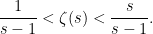 |
(13) |
In particular,  as approaches from above.
Moving on to , we can use the identity  , where
  is the real part of , to write,
Comparing the right hand side with the definition of , we get,
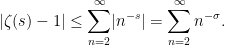
Lemma 6 The sum (1) converges absolutely at all with and satisfies the bound
where  .
.
The right-hand inequality here is just an application of (13). In particular, lemma 6 implies that is uniformly bounded on the half-plane  , any
, any  , with the bound
  . It also shows that
  uniformly as
  .
.
Next, the Euler product expansion (2) can be utilized to show that has no zeros on the open right half-plane . Applying the inequality  , which applies for all
  ,
,
with . Noting that the right hand side is just the reciprocal of the Euler product of  gives a lower bound.
Lemma 7 The zeta function is nonzero everywhere on the domain and satisfies the lower bound,
 |
(14) |
with .
The right-hand inequality here is another direct application of (13). Lemma 7 shows that is uniformly bounded away from zero on the half-plane , for any .
Expression (3) for the logarithm of the zeta function can be used to obtain further bounds. On the half-plane  , we use
  ,
,
So, we have obtained the following.
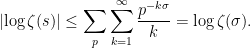
Lemma 8 The logarithm of the zeta function over  satisfies the bound
Applying this bound to  gives (14) as a special case.
Using  to denote the floor function, we can use the equality
  for
for  and each positive integer to rewrite the summation (1) as an integral
Substituting in the value for the first integral on the right hand side gives the following expression for the zeta function,
 |
(15) |
The idea is of that the integrand here is small in comparison to  , so that we can expect it to converge on a larger domain than the sum (1). In fact, as we will show, it is absolutely integrable on . As uniform limits of analytic functions are analytic, this will extend
  to an analytic function on this domain.
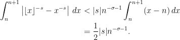
To bound the integrand in (15), note that has the derivative  with respect to . Using , this has norm
  and, as it is decreasing in , is bounded above by
  . Hence, the mean value theorem gives the inequality
which will be strict whenever is not an integer. For any positive integer , we have  on the interval
  and,
and,
Summing over and comparing with the definition of  gives a finite value, so we have proved the following.
Lemma 9 The zeta function extends to a meromorphic function on with a simple pole of residue at , and is given by the absolutely convergent integral (15). Furthermore, on this domain, it satisfies the bound
 |
(16) |
with .
The final inequality here is yet another application of (13). So, we have a bound for of size  on the right half-plane , for any
  . This is by no means optimal, and it can be improved to
  , with even better bounds given by the — as yet — unproven Lindelöf hypothesis.
Applying inequality (16) for real in the interval  shows that does not vanish,
Corollary 10  , so is nonzero, on the real line segment .
Interestingly, this bound is optimal, as  .
.
Elementary Extension of the Zeta Function
I will now describe an elementary method of analytically continuing the Riemann zeta function to the entire complex plane. Nothing in this section is required for the results discussed above, so can be skipped if required. The reason for including it here is to gain an intuitive understanding why the definition (1) of given on the half-plane should continue to all of , without using any `magic’ formulas such as Poisson summation or the functional equation. Instead, we can use the Euler-Maclaurin formula. Rather than just stating and applying this equation, I will derive it, as it is straightforward to do and gives a better understanding of why the zeta function necessarily extends to the complex plane.
We can apply a similar ideas to that which was used to express over by identity (15). To do this in more generality, I will look at a sum  for a smooth function . Some assumptions will be required on in order that the sums and integrals converge, so suppose that it is smooth and that its derivatives to all orders are integrable over
  . This is the case for the Riemann zeta function where
  .
.
For a differentiable function  defined on the interval
 ![{[0,1]}](https://s0.wp.com/latex.php?latex=%7B%5B0%2C1%5D%7D&bg=ffffff&fg=000000&s=0&c=20201002) , an integration by parts gives
, an integration by parts gives
for any constant  . The idea is to replace
  by
by  in this identity and sum over . In order that
  has average value over the unit interval, we will take
  . So, setting
  ,
,
 |
(17) |
with  denoting the fractional part of . That is
  on the interval . The hope here is that
  is sufficiently smaller then , so that the right-hand integral converges even when the sum on the left diverges.
We take this a step further and express the integral over as an integral over  . Again, consider a function defined on the unit interval and, choosing
  to be the integral of
  , another integration by parts gives
As has zero integral,  , so replacing by
  and summing over ,
Again, is only defined up to an arbitrary constant, so can be chosen to have zero integral over the unit interval.
We repeat this procedure  times and substitute into (17),
 |
(18) |
Here,  is defined as the integral of
  with constant of integration chosen such that it has zero integral over the unit interval,
From this definition, it can be seen that  where
where  are the Bernoulli polynomials,
  for Bernoulli numbers
  , and (18) is the Euler-Maclaurin formula.
In particular, the derivatives of can be computed as
with  denoting the rising factorial, which is just a polynomial in .
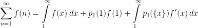
Taking for , the left hand side of identity (18) is and the first integral on the right is . Applying this to definition (1) of the zeta function,
 |
(19) |
As the integral on the right converges absolutely on  , and is an arbitrary positive integer, we have the analytic extension.
Theorem 11 The function defined on by (1) continues to a meromorphic function on with a single simple pole at of residue .
Furthermore, the integral on the right of (19) is uniformly bounded over  , any
, any  , and the terms are polynomials, so we have the following bound on the growth of the zeta function.
Lemma 12 For every real number  , there exists an
  such that
over , as  .
.
I purposefully did not put in any specific value for here, as the point is that the zeta function is polynomially bounded on each right half-plane and, in any case, there are more optimal values available from applying the functional equation.
Mellin Transforms
We show that the Mellin transform of a Schwartz function can be continued from the region to the entire complex plane, proving theorem 3. Choosing a positive integer  , write
This is bounded, and for  is just the remainder term in the Taylor polynomial approximation of . By Taylor’s theorem,
  as approaches . So,
  is absolutely integrable on
  and, hence,
  is a well-defined analytic function on this domain. The transform of the polynomial term can be computed,
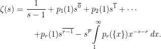
The Mellin transform of is then,
This statement holds for but, as the right hand side is a well-defined meromorphic function on , it extends to a meromorphic function on this domain. The poles arise from the  terms with the residue stated in theorem 3. By choosing arbitrarily large, we have the extension to the complex plane.
Poisson Summation
The second proof of the functional equation given by Riemann in his 1859 paper made use of the following identity of Jacobi,
For the Mellin transform version of the functional equation, we make use of the Poisson summation formula. To avoid having to explicitly write limits everywhere, the notation  is used to denote the sum as ranges over the integers
  .
.
Theorem 13 If  has Fourier transform then,
 |
(20) |
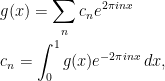
Jacobi’s identity is just a special case of this using  . The Poisson summation formula can be proved using Fourier series. The idea is that, for any Schwartz function , we can define a periodic
  by
by
 |
(21) |
Since and its derivatives vanish rapidly at  , this sum is uniformly convergent, with smooth limit. Writing out its Fourier expansion,
the Fourier coefficients can be evaluated,
Substituting into (21) proves theorem 13.
In practise, it is convenient to express the Poisson summation formula in a slightly more general way. For each fixed  , the Fourier transform of
  is equal to
  and, putting this in (20), gives the following alternative statement of Poisson summation.
Theorem 14 If has Fourier transform then, for any ,
 |
(22) |
The Functional Equation
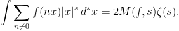
The proof of the functional equation starts with the following identity
Here, is any nonzero integer, is a Schwartz function on the reals, , and represents the Haar measure on the multiplicative group . The identity is achieved simply by substituting with  . Restricting to , we can sum over ,
 |
(23) |
What we would really like to do here is to simply substitute in (22) for the sum of  , substitute by
  in the integral, and immediately derive the functional equation (11). Unfortunately this leads to divergent sums and integrals. Instead, start by rearranging (22) as
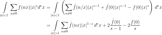
We will apply this to the integrand in (23), but only over the range with .
Here, we substituted for in the first term on the right hand side, and used the exact value for the integral in the other two terms. Using this in (23),
 |
(24) |
As vanishes faster than any power of at infinity, the sum  is absolutely convergent and also vanishes faster than any power of . The same statement holds for , so the integral in (24) is defined for all and is analytic. This extends to a meromorphic function on the complex plane with poles and residues as stated in theorem 4. Finally, noting that the Fourier transform of
  is
is  , the right hand side of (24) is unchanged if is replaced by
  and is replaced by , proving the functional equation (11).
A Note on Mellin Transforms
The Mellin transform was defined above as an integral over the real numbers (9), which deviates slightly from the more usual definition as an integral over the positive reals,
The reason for using the alternative definition is that we were interested in the functional equation relating it to the Fourier transform defined over the reals, so also required the Mellin transform to be defined with the same domain of integration. However, in doing so, we lose some properties, such as the existence of an inversion formula which, for the usual Mellin transform, is
for any fixed in the domain where the Mellin transform is absolutely integrable.
The transform defined by (9) is unchanged if is replaced by , so is not one-to-one and cannot be inverted. The best that can be done is to recover the even part of ,
An explanation for the non-invertibility of the Mellin transform defined over is that we did not consider the full set of characters. We only looked at characters of the form but, for example, this excludes the function  mapping positive reals to and negative reals to
  . More generally, for any and
  , a character
  can be defined by
 |
(25) |
It is immediate that this is a continuous map from the nonzero reals to satisfying 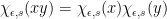 . In fact, it can shown that (25) gives the full set of characters on . The characters given by
  , which we made use of in the discussion above, are precisely those which are trivial on the roots of unity
  and are called unramified characters. Those given by
  are called ramified.
The Mellin transform with respect to an arbitrary character  is
is
The transform defined using the full set of characters can be inverted,
The argument given above, including the proof of the functional equation (11), could have been carried out with the full set of characters. In that case, the zeta function is replaced by
For the unramified characters, , this is the usual Riemann zeta function. For ramified characters, equals and the functional equation reduces to the trivial statement  . So, there was nothing to be gained by including ramified characters in the discussion.


 to denote the standard n-dimensional
 . By symmetric, we mean symmetric about the origin, so that
  is in A if and only
 denoting the Lebesgue integral on
  , and only consider real-valued processes. Any two processes are considered to be the same if they are equal
 ![{{\mathbb E}[1_{\{\tau < \infty\}}\lvert X_\tau\rvert\;\vert\mathcal{F}_\tau]}](https://s0.wp.com/latex.php?latex=%7B%7B%5Cmathbb+E%7D%5B1_%7B%5C%7B%5Ctau+%3C+%5Cinfty%5C%7D%7D%5Clvert+X_%5Ctau%5Crvert%5C%3B%5Cvert%5Cmathcal%7BF%7D_%5Ctau%5D%7D&bg=ffffff&fg=000000&s=0&c=20201002) is almost surely finite for each
is almost surely finite for each  . Then, there exists a unique optional process
  , referred to as the optional projection of X, satisfying
 ![\displaystyle 1_{\{\tau < \infty\}}{}^{\rm o}\!X_\tau={\mathbb E}[1_{\{\tau < \infty\}}X_\tau\,\vert\mathcal{F}_\tau]](https://s0.wp.com/latex.php?latex=%5Cdisplaystyle++1_%7B%5C%7B%5Ctau+%3C+%5Cinfty%5C%7D%7D%7B%7D%5E%7B%5Crm+o%7D%5C%21X_%5Ctau%3D%7B%5Cmathbb+E%7D%5B1_%7B%5C%7B%5Ctau+%3C+%5Cinfty%5C%7D%7DX_%5Ctau%5C%2C%5Cvert%5Cmathcal%7BF%7D_%5Ctau%5D+&bg=ffffff&fg=000000&s=0&c=20201002)
![{{\mathbb E}[1_{\{\tau < \infty\}}\lvert X_\tau\rvert\;\vert\mathcal{F}_{\tau-}]}](https://s0.wp.com/latex.php?latex=%7B%7B%5Cmathbb+E%7D%5B1_%7B%5C%7B%5Ctau+%3C+%5Cinfty%5C%7D%7D%5Clvert+X_%5Ctau%5Crvert%5C%3B%5Cvert%5Cmathcal%7BF%7D_%7B%5Ctau-%7D%5D%7D&bg=ffffff&fg=000000&s=0&c=20201002) is almost surely finite for each
is almost surely finite for each  , referred to as the predictable projection of X, satisfying
 ![\displaystyle 1_{\{\tau < \infty\}}{}^{\rm p}\!X_\tau={\mathbb E}[1_{\{\tau < \infty\}}X_\tau\,\vert\mathcal{F}_{\tau-}]](https://s0.wp.com/latex.php?latex=%5Cdisplaystyle++1_%7B%5C%7B%5Ctau+%3C+%5Cinfty%5C%7D%7D%7B%7D%5E%7B%5Crm+p%7D%5C%21X_%5Ctau%3D%7B%5Cmathbb+E%7D%5B1_%7B%5C%7B%5Ctau+%3C+%5Cinfty%5C%7D%7DX_%5Ctau%5C%2C%5Cvert%5Cmathcal%7BF%7D_%7B%5Ctau-%7D%5D+&bg=ffffff&fg=000000&s=0&c=20201002)
 decreasing to a limit
  ,
,  almost-surely tends to
  . However, even if we can prove this for every possible decreasing sequence
  , it does not follow that X is right-continuous. As a counterexample, if
  is any continuously distributed random time, then the process
  is not right-continuous. However, so long as the distribution of
  . Two processes are considered to be the same if they are equal
  in probability, for each uniformly bounded sequence
  of stopping times decreasing to a limit
  converges in probability, for each uniformly bounded decreasing sequence
  . In light of such examples, it is even more remarkable that right-continuity and the existence of left and right limits can be determined by just looking at convergence in probability along monotonic sequences of stopping times. Theorem
  and a subset S of
  . The projection
  is the set of
  such that there exists a
  with
with  . We can ask whether there exists a map
 . From the definition of the projection, values of
  satisfying this exist for each individual
  . By invoking the
  , with
  denoting the
  . Also, less obviously, the underlying probability space should be
  by setting
  for
for  for which
  precisely when
 ![{[\tau]}](https://s0.wp.com/latex.php?latex=%7B%5B%5Ctau%5D%7D&bg=ffffff&fg=000000&s=0&c=20201002) , is defined to be the set of
, is defined to be the set of  with
with  . The property that
 ![{[\tau]\subseteq S}](https://s0.wp.com/latex.php?latex=%7B%5B%5Ctau%5D%5Csubseteq+S%7D&bg=ffffff&fg=000000&s=0&c=20201002) . With this notation, the measurable selection theorem is as follows.
. With this notation, the measurable selection theorem is as follows.
 , there exists a measurable
  such that
 , so the
  and a measurable function,
  , does there exist a measurable right-inverse on the image of
  , from
  to
to  such that
  . In the case where
  , Theorem
  then
then  . However, completeness is not actually required for the following result. All processes are assumed to be real valued, or take values in the extended reals
  .
.
 :
:  as
as  -measurable
 .
.  :
:  {
{ }.
}.  , is the sigma-algebra on
  , was defined earlier in these notes as the sigma-algebra generated by the adapted and right-continuous processes. Then, a stochastic process is optional if it is
  -measurable
 then
then  .
.  is used to denote the projection from the
  of sets A and B onto B. That is,
  . As is standard,
  is the
  denotes the
  onto
onto  all project onto the whole of
  and
and  , Theorem
  is assumed to be complete, and stochastic processes are taken to be real-valued, or take values in the extended reals
  then
then  is measurable.
  then, for each real K,
  if and only if
  for some
  . Hence,
 ![\displaystyle U^{-1}\left((K,\infty]\right)=\pi_\Omega\left((S\times\Omega)\cap X^{-1}\left((K,\infty]\right)\right).](https://s0.wp.com/latex.php?latex=%5Cdisplaystyle++U%5E%7B-1%7D%5Cleft%28%28K%2C%5Cinfty%5D%5Cright%29%3D%5Cpi_%5COmega%5Cleft%28%28S%5Ctimes%5COmega%29%5Ccap+X%5E%7B-1%7D%5Cleft%28%28K%2C%5Cinfty%5D%5Cright%29%5Cright%29.+&bg=ffffff&fg=000000&s=0&c=20201002)
 and, as sets of the form
 ![{(K,\infty]}](https://s0.wp.com/latex.php?latex=%7B%28K%2C%5Cinfty%5D%7D&bg=ffffff&fg=000000&s=0&c=20201002) generate the Borel sigma-algebra on
generate the Borel sigma-algebra on  , U is
  is also jointly measurable.
 . Then, the conditional expectation of X is written as,
 ![\displaystyle Y_t={\mathbb E}[X_t\;\vert\mathcal{F}_{t-}]{\rm\ \ (a.s.)}](https://s0.wp.com/latex.php?latex=%5Cdisplaystyle++Y_t%3D%7B%5Cmathbb+E%7D%5BX_t%5C%3B%5Cvert%5Cmathcal%7BF%7D_%7Bt-%7D%5D%7B%5Crm%5C+%5C+%28a.s.%29%7D+&bg=ffffff&fg=000000&s=0&c=20201002)
 is used in place of
  .
.
![\displaystyle {}^{\rm p}\!X_t={\mathbb E}[X_t\;\vert\mathcal{F}_{t-}]{\rm\ \ (a.s.)}](https://s0.wp.com/latex.php?latex=%5Cdisplaystyle++%7B%7D%5E%7B%5Crm+p%7D%5C%21X_t%3D%7B%5Cmathbb+E%7D%5BX_t%5C%3B%5Cvert%5Cmathcal%7BF%7D_%7Bt-%7D%5D%7B%5Crm%5C+%5C+%28a.s.%29%7D+&bg=ffffff&fg=000000&s=0&c=20201002)
 is the left-limits of the cadlag martingale
 ![{M_t={\mathbb E}[U\;\vert\mathcal{F}_t]}](https://s0.wp.com/latex.php?latex=%7BM_t%3D%7B%5Cmathbb+E%7D%5BU%5C%3B%5Cvert%5Cmathcal%7BF%7D_t%5D%7D&bg=ffffff&fg=000000&s=0&c=20201002) , so
, so 