Localization

Special classes of processes, such as martingales, are very important to the study of stochastic calculus. In many cases, however, processes under consideration `almost’ satisfy the martingale property, but are not actually martingales. This occurs, for example, when taking limits or stochastic integrals with respect to martingales. It is necessary to generalize the martingale concept to that of local martingales. More generally, localization is a method of extending a given property to a larger class of processes. In this post I mention a few definitions and simple results concerning localization, and look more closely at local martingales in the next post.

Definition 1 Let P be a class of stochastic processes. Then, a process X is locally in P if there exists a sequence of stopping times ${\tau_n\uparrow\infty}$ such that the stopped processes

$\displaystyle 1_{\{\tau_n>0\}}X^{\tau_n}$

are in P. The sequence ${\tau_n}$ is called a localizing sequence for X (w.r.t. P).

I write ${P_{\rm loc}}$ for the processes locally in P. Choosing the sequence ${\tau_n\equiv\infty}$ of stopping times shows that ${P\subseteq P_{\rm loc}}$ . A class of processes is said to be stable if ${1_{\{\tau>0\}}X^\tau}$ is in P whenever X is, for all stopping times ${\tau}$ . For example, the optional stopping theorem shows that the classes of cadlag martingales, cadlag submartingales and cadlag supermartingales are all stable.

Definition 2 A process is a

a local martingale if it is locally in the class of cadlag martingales.

a local submartingale if it is locally in the class of cadlag submartingales.

a local supermartingale if it is locally in the class of cadlag supermartingales.

Continue reading “Localization” →

Class (D) Processes

A stochastic process X is said to be uniformly integrable if the set of random variables ${\{X_t\colon t\in{\mathbb R}_+\}}$ is uniformly integrable. However, even if this is the case, it does not follow that the set of values of the process sampled at arbitrary stopping times is uniformly integrable.

For the case of a cadlag martingale X, optional sampling can be used. If ${t\ge 0}$ is any fixed time then this says that ${X_\tau={\mathbb E}[X_t\mid\mathcal{F}_\tau]}$ for stopping times ${\tau\le t}$ . As sets of conditional expectations of a random variable are uniformly integrable, the following result holds.

Lemma 1 Let X be a cadlag martingale. Then, for each ${t\ge 0}$ , the set

$\displaystyle \{X_\tau\colon\tau\le t\text{\ is\ a\ stopping\ time}\}$

is uniformly integrable.

This suggests the following generalized concepts of uniform integrability for stochastic processes.

Definition 2 Let X be a jointly measurable stochastic process. Then, it is

of class (D) if ${\{X_\tau\colon\tau<\infty\text{ is a stopping time}\}}$ is uniformly integrable.

of class (DL) if, for each ${t\ge 0}$ , ${\{X_\tau\colon\tau\le t\text{ is a stopping time}\}}$ is uniformly integrable.

Continue reading “Class (D) Processes” →

Martingale Inequalities

Martingale inequalities are an important subject in the study of stochastic processes. The subject of this post is Doob’s inequalities which bound the distribution of the maximum value of a martingale in terms of its terminal distribution, and is a consequence of the optional sampling theorem. We work with respect to a filtered probability space ${(\Omega,\mathcal{F},\{\mathcal{F}_t\}_{t\ge 0},{\mathbb P})}$ . The absolute maximum process of a martingale is denoted by ${X^*_t\equiv\sup_{s\le t}\vert X_s\vert}$ . For any real number ${p\ge 1}$ , the ${L^p}$ -norm of a random variable ${Z}$ is

$\displaystyle \Vert Z\Vert_p\equiv{\mathbb E}[|Z|^p]^{1/p}.$

Then, Doob’s inequalities bound the distribution of the maximum of a martingale by the ${L^1}$ -norm of its terminal value, and bound the ${L^p}$ -norm of its maximum by the ${L^p}$ -norm of its terminal value for all ${p>1}$ .

Theorem 1 Let ${X}$ be a cadlag martingale and ${t>0}$ . Then

for every ${K>0}$ ,
$\displaystyle {\mathbb P}(X^*_t\ge K)\le\frac{\lVert X_t\rVert_1}{K}.$

for every ${p>1}$ ,
$\displaystyle \lVert X^*_t\rVert_p\le \frac{p}{p-1}\Vert X_t\Vert_p.$

$\displaystyle \lVert X^*_t\rVert_1\le\frac e{e-1}{\mathbb E}\left[\lvert X_t\rvert \log\lvert X_t\rvert+1\right].$

Continue reading “Martingale Inequalities” →

Martingale Convergence

The martingale property is strong enough to ensure that, under relatively weak conditions, we are guaranteed convergence of the processes as time goes to infinity. In a previous post, I used Doob’s upcrossing inequality to show that, with probability one, discrete-time martingales will converge at infinity under the extra condition of ${L^1}$ -boundedness. Here, I consider continuous-time martingales. This is a more general situation, because it considers limits as time runs through the uncountably infinite set of positive reals instead of the countable set of positive integer times. Although these results can also be proven in a similar way by counting the upcrossings of a process, I instead show how they follow directly from the existence of cadlag modifications. We work with respect to a complete filtered probability space ${(\Omega,\mathcal{F},\{\mathcal{F}_t\}_{t\ge 0},{\mathbb P})}$ .

Recall that a stochastic process ${X}$ is ${L^1}$ -bounded if the set ${\{X_t\colon t\in{\mathbb R}_+\}}$ is ${L^1}$ -bounded. That is, ${{\mathbb E}|X_t|}$ is bounded above by some finite value as ${t}$ runs through the positive reals.

Theorem 1 Let ${X}$ be a cadlag and ${L^1}$ -bounded martingale (or submartingale, or supermartingale). Then, the limit ${X_\infty=\lim_{t\rightarrow\infty}X_t}$ exists and is finite, with probability one.

Continue reading “Martingale Convergence” →

Optional Sampling

Doob’s optional sampling theorem states that the properties of martingales, submartingales and supermartingales generalize to stopping times. For simple stopping times, which take only finitely many values in ${{\mathbb R}_+}$ , the argument is a relatively basic application of elementary integrals. For simple stopping times ${\sigma\le\tau}$ , the stochastic interval ${(\sigma,\tau]}$ and its indicator function ${1_{(\sigma,\tau]}}$ are elementary predictable. For any submartingale ${X}$ , the properties of elementary integrals give the inequality

$\displaystyle {\mathbb E}\left[X_\tau-X_\sigma\right]={\mathbb E}\left[\int_0^\infty 1_{(\sigma,\tau]}\,dX\right]\ge 0.$

(1)

For a set ${A\in \mathcal{F}_\sigma}$ the following

$\displaystyle \sigma^\prime(\omega)=\begin{cases} \sigma(\omega),&\textrm{if }\omega\in A,\\ \tau(\omega),&\textrm{otherwise}, \end{cases}$

is easily seen to be a stopping time. Replacing ${\sigma}$ by ${\sigma^\prime}$ extends inequality (1) to the following,

$\displaystyle {\mathbb E}\left[1_A(X_\tau-X_\sigma)\right]={\mathbb E}\left[X_\tau-X_{\sigma^\prime}\right]\ge 0.$

(2)

As this inequality holds for all sets ${A\in\mathcal{F}_\sigma}$ it implies the extension of the submartingale property ${X_\sigma\le{\mathbb E}[X_\tau\vert\mathcal{F}_\sigma]}$ to the random times. This argument applies to all simple stopping times, and is sufficient to prove the optional sampling result for discrete time submartingales. In continuous time, the additional hypothesis that the process is right-continuous is required. Then, the result follows by taking limits of simple stopping times.

Theorem 1 Let ${\sigma\le\tau}$ be bounded stopping times. For any cadlag martingale, submartingale or supermartingale ${X}$ , the random variables ${X_\sigma, X_\tau}$ are integrable and the following are satisfied.

If ${X}$ is a martingale then, ${X_\sigma={\mathbb E}\left[X_{\tau}\vert\mathcal{F}_\sigma\right].}$

If ${X}$ is a submartingale then, ${X_\sigma\le{\mathbb E}\left[X_{\tau}\vert\mathcal{F}_\sigma\right].}$

If ${X}$ is a supermartingale then, ${X_\sigma\ge{\mathbb E}\left[X_{\tau}\vert\mathcal{F}_\sigma\right].}$

Continue reading “Optional Sampling” →

Cadlag Modifications

As was mentioned in the initial post of these stochastic calculus notes, it is important to choose good versions of stochastic processes. In some cases, such as with Brownian motion, it is possible to explicitly construct the process to be continuous. However, in many more cases, it is necessary to appeal to more general results to assure the existence of such modifications.

The theorem below guarantees that many of the processes studied in stochastic calculus have a right-continuous version and, furthermore, these versions necessarily have left limits everywhere. Such processes are known as càdlàg from the French for “continu à droite, limites à gauche” (I often drop the accents, as seems common). Alternative terms used to refer to a cadlag process are rcll (right-continuous with left limits), R-process and right process. For a cadlag process ${X}$ , the left limit at any time ${t>0}$ is denoted by ${X_{t-}}$ (and ${X_{0-}\equiv X_0}$ ). The jump at time ${t}$ is denoted by ${\Delta X_t=X_t-X_{t-}}$ .

We work with respect to a complete filtered probability space ${(\Omega,\mathcal{F},\{\mathcal{F}_t\}_{t\ge 0},{\mathbb P})}$ .

Theorem 1 below provides us with cadlag versions under the condition that elementary integrals of the processes cannot, in a sense, get too large. Recall that elementary predictable processes are of the form

$\displaystyle \xi=Z_01_{\{t=0\}}+\sum_{k=1}^nZ_k1_{\{s_k<t\le t_k\}}$

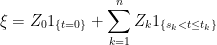
for times ${s_k<t_k}$ , ${\mathcal{F}_0}$ -measurable random variable ${Z_0}$ and ${\mathcal{F}_{s_k}}$ -measurable random variables ${Z_k}$ . Its integral with respect to a stochastic process ${X}$ is

$\displaystyle \int_0^t \xi\,dX=\sum_{k=1}^nZ_k(X_{t_k\wedge t}-X_{s_{k}\wedge t}).$

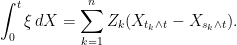
An elementary predictable set is a subset of ${{\mathbb R}_+\times\Omega}$ which is a finite union of sets of the form ${\{0\}\times F}$ for ${F\in\mathcal{F}_0}$ and ${(s,t]\times F}$ for nonnegative reals ${s<t}$ and ${F\in\mathcal{F}_s}$ . Then, a process is an indicator function ${1_A}$ of some elementary predictable set ${A}$ if and only if it is elementary predictable and takes values in ${\{0,1\}}$ .

The following theorem guarantees the existence of cadlag versions for many types of processes. The first statement applies in particular to martingales, submartingales and supermartingales, whereas the second statement is important for the study of general semimartingales.

Theorem 1 Let X be an adapted stochastic process which is right-continuous in probability and such that either of the following conditions holds. Then, it has a cadlag version.

X is integrable and, for every ${t\in{\mathbb R}_+}$ ,
$\displaystyle \left\{{\mathbb E}\left[\int_0^t1_A\,dX\right]\colon A\textrm{ is elementary}\right\}$

is bounded.

For every ${t\in{\mathbb R}_+}$ the set
$\displaystyle \left\{\int_0^t1_A\,dX\colon A\textrm{ is elementary}\right\}$

is bounded in probability.

Continue reading “Cadlag Modifications” →

Upcrossings, Downcrossings, and Martingale Convergence

The number of times that a process passes upwards or downwards through an interval is refered to as the number of upcrossings and respectively the number of downcrossings of the process.

Consider a process ${X_t}$ whose time index ${t}$ runs through an index set ${\mathbb{T}\subseteq{\mathbb R}}$ . For real numbers ${a<b}$ , the number of upcrossings of ${X}$ across the interval ${[a,b]}$ is the supremum of the nonnegative integers ${n}$ such that there exists times ${s_k,t_k\in\mathbb{T}}$ satisfying

$\displaystyle s_1<t_1<s_2<t_2<\cdots<s_n<t_n$

(1)

and for which ${X_{s_k}\le a<b\le X_{t_k}}$ . The number of upcrossings is denoted by ${U[a,b]}$ , which is either a nonnegative integer or is infinite. Similarly, the number of downcrossings, denoted by ${D[a,b]}$ , is the supremum of the nonnegative integers ${n}$ such that there are times ${s_k,t_k\in\mathbb{T}}$ satisfying (1) and such that ${X_{s_k}\ge b>a\ge X_{t_k}}$ .

Note that between any two upcrossings there is a downcrossing and, similarly, between any two downcrossings there is an upcrossing. It follows that ${U[a,b]}$ and ${D[a,b]}$ can differ by at most 1, and they are either both finite or both infinite.

The significance of the upcrossings of a process to convergence results is due to the following criterion for convergence of a sequence.

Theorem 1 A sequence ${x_1,x_2,\ldots}$ converges to a limit in the extended real numbers if and only if the number of upcrossings ${U[a,b]}$ is finite for all ${a<b}$ .

Continue reading “Upcrossings, Downcrossings, and Martingale Convergence” →

Martingales and Elementary Integrals

A martingale is a stochastic process which stays the same, on average. That is, the expected future value conditional on the present is equal to the current value. Examples include the wealth of a gambler as a function of time, assuming that he is playing a fair game. The canonical example of a continuous time martingale is Brownian motion and, in discrete time, a symmetric random walk is a martingale. As always, we work with respect to a filtered probability space ${(\Omega,\mathcal{F},\{\mathcal{F}_t\}_{t\ge 0},{\mathbb P})}$ . A process ${X}$ is said to be integrable if the random variables ${X_t}$ are integrable, so that ${{\mathbb E}[\vert X_t\vert]<\infty}$ .

Definition 1 A martingale, ${X}$ , is an integrable process satisfying

$\displaystyle X_s={\mathbb E}[X_t\mid\mathcal{F}_s]$

for all ${s<t\in{\mathbb R}_+}$ .

Continue reading “Martingales and Elementary Integrals” →

	Anonymous on Spitzer’s Formula
	Anonymous on Spitzer’s Formula
	Anonymous on Brownian Bridges
	Anonymous on Spitzer’s Formula
	Anonymous on Spitzer’s Formula
	Anonymous on Spitzer’s Formula
	Anonymous on Spitzer’s Formula
	Anonymous on Spitzer’s Formula
	Anonymous on Spitzer’s Formula
	Anonymous on Spitzer’s Formula