
For stochastic processes in discrete time, the Doob decomposition uniquely decomposes any integrable process into the sum of a martingale and a predictable process. If 

![{M_{n-1}={\mathbb E}[M_n\vert\mathcal{F}_{n-1}]}](https://s0.wp.com/latex.php?latex=%7BM_%7Bn-1%7D%3D%7B%5Cmathbb+E%7D%5BM_n%5Cvert%5Cmathcal%7BF%7D_%7Bn-1%7D%5D%7D&bg=ffffff&fg=000000&s=0&c=20201002)


![\displaystyle A_n-A_{n-1}={\mathbb E}[A_n-A_{n-1}\vert\mathcal{F}_{n-1}]={\mathbb E}[X_n-X_{n-1}\vert\mathcal{F}_{n-1}].](https://s0.wp.com/latex.php?latex=%5Cdisplaystyle++A_n-A_%7Bn-1%7D%3D%7B%5Cmathbb+E%7D%5BA_n-A_%7Bn-1%7D%5Cvert%5Cmathcal%7BF%7D_%7Bn-1%7D%5D%3D%7B%5Cmathbb+E%7D%5BX_n-X_%7Bn-1%7D%5Cvert%5Cmathcal%7BF%7D_%7Bn-1%7D%5D.+&bg=ffffff&fg=000000&s=0&c=20201002)
Then it is possible to write A and M as
![\displaystyle \setlength\arraycolsep{2pt} \begin{array}{rl} \displaystyle A_n&\displaystyle=\sum_{k=1}^n{\mathbb E}[X_k-X_{k-1}\vert\mathcal{F}_{k-1}],\smallskip\\ \displaystyle M_n&\displaystyle=X_n-A_n. \end{array}](https://s0.wp.com/latex.php?latex=%5Cdisplaystyle++%5Csetlength%5Carraycolsep%7B2pt%7D+%5Cbegin%7Barray%7D%7Brl%7D+%5Cdisplaystyle+A_n%26%5Cdisplaystyle%3D%5Csum_%7Bk%3D1%7D%5En%7B%5Cmathbb+E%7D%5BX_k-X_%7Bk-1%7D%5Cvert%5Cmathcal%7BF%7D_%7Bk-1%7D%5D%2C%5Csmallskip%5C%5C+%5Cdisplaystyle+M_n%26%5Cdisplaystyle%3DX_n-A_n.+%5Cend%7Barray%7D+&bg=ffffff&fg=000000&s=0&c=20201002) |
(1) |
So, the Doob decomposition is unique and, conversely, the processes A and M constructed according to equation (1) can be seen to be respectively, a predictable process starting from zero and a martingale. For many purposes, this allows us to reduce problems concerning processes in discrete time to simpler statements about martingales and separately about predictable processes. In the case where X is a submartingale then things reduce further as, in this case, A will be an increasing process.
The situation is considerably more complicated when looking at processes in continuous time. The extension of the Doob decomposition to continuous time processes, known as the Doob-Meyer decomposition, was an important result historically in the development of stochastic calculus. First, we would usually restrict attention to sufficiently nice modifications of the processes and, in particular, suppose that X is cadlag. When attempting an analogous decomposition to the one above, it is not immediately clear what should be meant by the predictable component. The continuous time predictable processes are defined to be the set of all processes which are measurable with respect to the predictable sigma algebra, which is the sigma algebra generated by the space of processes which are adapted and continuous (or, equivalently, left-continuous). In particular, all continuous and adapted processes are predictable but, due to the existence of continuous martingales such as Brownian motion, this means that decompositions as sums of martingales and predictable processes are not unique. It is therefore necessary to impose further conditions on the term A in the decomposition. It turns out that we obtain unique decompositions if, in addition to being predictable, A is required to be cadlag with locally finite variation (an FV process). The processes which can be decomposed into a local martingale and a predictable FV process are known as special semimartingales. This is precisely the space of locally integrable semimartingales. As usual, we work with respect to a complete filtered probability space 
Theorem 1 For a process X, the following are equivalent.
- X is a locally integrable semimartingale.
- X decomposes as
(2) for a local martingale M and predictable FV process A.
Furthermore, choosing

Theorem 1 is a general version of the Doob-Meyer decomposition. However, the name `Doob-Meyer decomposition’ is often used to specifically refer to the important special case where X is a submartingale. Historically, the theorem was first stated and proved for that case, and I will look at the decomposition for submartingales in more detail in a later post. Compare with the Bichteler-Dellacherie theorem, which says that a process is a semimartingale if and only if it decomposes as the sum of a local martingale and an FV process. Unfortunately, that decomposition is not unique. By Theorem 1, uniqueness is obtained by requiring the finite variation term to also be predictable, at the cost of restricting the result to apply only to locally integrable processes. Compare also with the unique decomposition of continuous semimartingales into a continuous local martingale and a continuous FV process. When looking at non-continuous processes, predictable FV processes are the correct generalisation of continuous FV processes.
The proof of Theorem 1 follows almost immediately from the proof of the Bichteler-Dellacherie theorem described in these notes, together with the classification of predictable FV processes. That is, we orthogonally project the process X onto a local martingale M, then show that 

![{[0,\tau]}](https://s0.wp.com/latex.php?latex=%7B%5B0%2C%5Ctau%5D%7D&bg=ffffff&fg=000000&s=0&c=20201002)

Lemma 2 If M is a local martingale, A is a predictable FV process and
then
for all stopping times
.
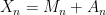
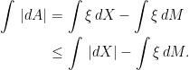
![\displaystyle {\mathbb E}\left[\int_0^\tau\,\vert dA\vert\right] \le {\mathbb E}\left[\int_0^\tau\,\vert dX\vert\right]](https://s0.wp.com/latex.php?latex=%5Cdisplaystyle++%7B%5Cmathbb+E%7D%5Cleft%5B%5Cint_0%5E%5Ctau%5C%2C%5Cvert+dA%5Cvert%5Cright%5D+%5Cle+%7B%5Cmathbb+E%7D%5Cleft%5B%5Cint_0%5E%5Ctau%5C%2C%5Cvert+dX%5Cvert%5Cright%5D+&bg=ffffff&fg=000000&s=0&c=20201002)
Proof: As A is a predictable FV process, there exists a predictable process 


As 


![\displaystyle {\mathbb E}\left[\int_0^{\tau\wedge\tau_n}\,\vert dA\vert\right]\le{\mathbb E}\left[\int_0^{\tau\wedge\tau_n}\,\vert dX\vert\right].](https://s0.wp.com/latex.php?latex=%5Cdisplaystyle++%7B%5Cmathbb+E%7D%5Cleft%5B%5Cint_0%5E%7B%5Ctau%5Cwedge%5Ctau_n%7D%5C%2C%5Cvert+dA%5Cvert%5Cright%5D%5Cle%7B%5Cmathbb+E%7D%5Cleft%5B%5Cint_0%5E%7B%5Ctau%5Cwedge%5Ctau_n%7D%5C%2C%5Cvert+dX%5Cvert%5Cright%5D.+&bg=ffffff&fg=000000&s=0&c=20201002)
Letting n go to infinity and using monotone convergence gives the result. ⬜
With this lemma out of the way, we can now give the proof of Theorem 1.
Proof of Theorem 1: If 


Next, sums of local martingales and FV processes are semimartingales. Also, local martingales are locally integrable, as are cadlag predictable processes. So, the first statement follows from the second. In the case where X is a locally square-integrable semimartingale, the reverse implication follows quickly from previous results of these notes. As in the proof of the Bichteler-Dellacherie theorem, any such X decomposes as 
![{[A,N]}](https://s0.wp.com/latex.php?latex=%7B%5BA%2CN%5D%7D&bg=ffffff&fg=000000&s=0&c=20201002)
It just remains to show that decomposition (2) exists for all locally integrable semimartingales X. Choose a sequence of stopping times
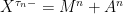
are locally square integrable. For example, taking 


for locally square integrable martingales 


Choosing m,n and a stopping time 
![\displaystyle \setlength\arraycolsep{2pt} \begin{array}{rl} \displaystyle{\mathbb E}\left[\sup_{t\le\sigma}\vert A^m_t-A^n_t\vert\right]&\displaystyle\le{\mathbb E}\left[\int_0^\sigma\,\vert d(A^m-A^n)\vert\right]\smallskip\\ &\displaystyle\le{\mathbb E}\left[\int_0^\sigma\,\vert d(X^{\tau_m-}-X^{\tau_n-})\vert\right]\smallskip\\ &\displaystyle\le{\mathbb E}\left[1_{\{\tau_m\wedge\tau_n=\sigma\}}\vert\Delta X_\sigma\vert\right]. \end{array}](https://s0.wp.com/latex.php?latex=%5Cdisplaystyle++%5Csetlength%5Carraycolsep%7B2pt%7D+%5Cbegin%7Barray%7D%7Brl%7D+%5Cdisplaystyle%7B%5Cmathbb+E%7D%5Cleft%5B%5Csup_%7Bt%5Cle%5Csigma%7D%5Cvert+A%5Em_t-A%5En_t%5Cvert%5Cright%5D%26%5Cdisplaystyle%5Cle%7B%5Cmathbb+E%7D%5Cleft%5B%5Cint_0%5E%5Csigma%5C%2C%5Cvert+d%28A%5Em-A%5En%29%5Cvert%5Cright%5D%5Csmallskip%5C%5C+%26%5Cdisplaystyle%5Cle%7B%5Cmathbb+E%7D%5Cleft%5B%5Cint_0%5E%5Csigma%5C%2C%5Cvert+d%28X%5E%7B%5Ctau_m-%7D-X%5E%7B%5Ctau_n-%7D%29%5Cvert%5Cright%5D%5Csmallskip%5C%5C+%26%5Cdisplaystyle%5Cle%7B%5Cmathbb+E%7D%5Cleft%5B1_%7B%5C%7B%5Ctau_m%5Cwedge%5Ctau_n%3D%5Csigma%5C%7D%7D%5Cvert%5CDelta+X_%5Csigma%5Cvert%5Cright%5D.+%5Cend%7Barray%7D+&bg=ffffff&fg=000000&s=0&c=20201002)
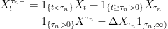
As X is locally integrable, there exists a sequence of finite stopping times 

![\displaystyle \setlength\arraycolsep{2pt} \begin{array}{rl} \displaystyle{\mathbb E}\left[\sup_{t\le\sigma_k\wedge\tau_m\wedge\tau_n}\vert A^m_t-A^n_t\vert\right]&\displaystyle\le{\mathbb E}\left[1_{\{\tau_m\wedge\tau_n\le\sigma_k\}}\vert\Delta X_{\sigma_k}\vert\right]\smallskip\\ &\rightarrow0 \end{array}](https://s0.wp.com/latex.php?latex=%5Cdisplaystyle++%5Csetlength%5Carraycolsep%7B2pt%7D+%5Cbegin%7Barray%7D%7Brl%7D+%5Cdisplaystyle%7B%5Cmathbb+E%7D%5Cleft%5B%5Csup_%7Bt%5Cle%5Csigma_k%5Cwedge%5Ctau_m%5Cwedge%5Ctau_n%7D%5Cvert+A%5Em_t-A%5En_t%5Cvert%5Cright%5D%26%5Cdisplaystyle%5Cle%7B%5Cmathbb+E%7D%5Cleft%5B1_%7B%5C%7B%5Ctau_m%5Cwedge%5Ctau_n%5Cle%5Csigma_k%5C%7D%7D%5Cvert%5CDelta+X_%7B%5Csigma_k%7D%5Cvert%5Cright%5D%5Csmallskip%5C%5C+%26%5Crightarrow0+%5Cend%7Barray%7D+&bg=ffffff&fg=000000&s=0&c=20201002)
as m,n go to infinity. So 

![\displaystyle {\mathbb E}\left[\int_0^{\sigma_k\wedge\tau_n}\,\vert d(A-A^n)\vert\right]\le\lim_{m\rightarrow\infty}{\mathbb E}\left[\int_0^{\sigma_k\wedge\tau_n}\,\vert d(A^m-A^n)\vert\right]\rightarrow0](https://s0.wp.com/latex.php?latex=%5Cdisplaystyle++%7B%5Cmathbb+E%7D%5Cleft%5B%5Cint_0%5E%7B%5Csigma_k%5Cwedge%5Ctau_n%7D%5C%2C%5Cvert+d%28A-A%5En%29%5Cvert%5Cright%5D%5Cle%5Clim_%7Bm%5Crightarrow%5Cinfty%7D%7B%5Cmathbb+E%7D%5Cleft%5B%5Cint_0%5E%7B%5Csigma_k%5Cwedge%5Ctau_n%7D%5C%2C%5Cvert+d%28A%5Em-A%5En%29%5Cvert%5Cright%5D%5Crightarrow0+&bg=ffffff&fg=000000&s=0&c=20201002)
as n goes to infinity. In particular, A has finite variation on the range ![{[0,\sigma_k\wedge\tau_n]}](https://s0.wp.com/latex.php?latex=%7B%5B0%2C%5Csigma_k%5Cwedge%5Ctau_n%5D%7D&bg=ffffff&fg=000000&s=0&c=20201002)


![{[0,\tau_m\wedge\tau_n]}](https://s0.wp.com/latex.php?latex=%7B%5B0%2C%5Ctau_m%5Cwedge%5Ctau_n%5D%7D&bg=ffffff&fg=000000&s=0&c=20201002)

Special Semimartingales as Integrators
Having established the canonical decomposition (2) for special semimartingales, we can now move on to stochastic integration. In fact, the decomposition is particularly well behaved under integration, inasmuch as it commutes with the integral. The integral of a predictable process with respect to a special semimartingale can be split up into separate integrals with respect to the martingale and predictable FV parts. This compatibility of stochastic integration with semimartingale decompositions was previously seen in the special case of continuous semimartingales. However, for noncontinuous semimartingales, there is one restriction for this to hold. We are only guaranteed that the integrals with respect to the separate components are well-defined if it is assumed that the integral is itself locally integrable.
In some approaches, the compatibility of integration with the canonical decomposition is used in the construction of the stochastic integral. This is the case, for example, in Protter (Stochastic Integration and Differential Equations). There, a predictable process
Compare Theorem 3 with the more general decomposition of a semimartingale into local martingale and FV terms given by the Bichteler-Dellacherie theorem. In that case, it is possible for a predictable process 
Theorem 3 Let X be a special semimartingale and
is a local martingale.
is locally integrable.
Then,
(3) is the unique decomposition of

Proof: 1 ⇒ 2: As 


However, 


Integrating 


2 ⇒ 3: By assumption, 
![{[N]}](https://s0.wp.com/latex.php?latex=%7B%5BN%5D%7D&bg=ffffff&fg=000000&s=0&c=20201002)
![{\Delta[N]=(\Delta N)^2}](https://s0.wp.com/latex.php?latex=%7B%5CDelta%5BN%5D%3D%28%5CDelta+N%29%5E2%7D&bg=ffffff&fg=000000&s=0&c=20201002)
![{[N]^{1/2}}](https://s0.wp.com/latex.php?latex=%7B%5BN%5D%5E%7B1%2F2%7D%7D&bg=ffffff&fg=000000&s=0&c=20201002)

![\displaystyle \sqrt{\int\xi^2\,d[M]}+\int\vert\xi\vert\,\vert dA\vert=\sqrt{[N]}+\int\vert\xi\vert\,\vert dA\vert](https://s0.wp.com/latex.php?latex=%5Cdisplaystyle++%5Csqrt%7B%5Cint%5Cxi%5E2%5C%2Cd%5BM%5D%7D%2B%5Cint%5Cvert%5Cxi%5Cvert%5C%2C%5Cvert+dA%5Cvert%3D%5Csqrt%7B%5BN%5D%7D%2B%5Cint%5Cvert%5Cxi%5Cvert%5C%2C%5Cvert+dA%5Cvert+&bg=ffffff&fg=000000&s=0&c=20201002)
is locally integrable.
3 ⇒ 1: It was previously shown that, as a consequence of the Burkholder-Davis-Gundy inequality, local integrability of ![{\left(\int\xi^2\,d[M]\right)^{1/2}}](https://s0.wp.com/latex.php?latex=%7B%5Cleft%28%5Cint%5Cxi%5E2%5C%2Cd%5BM%5D%5Cright%29%5E%7B1%2F2%7D%7D&bg=ffffff&fg=000000&s=0&c=20201002)
is locally integrable as required. ⬜

Hi,
There is a notation that I don’t fully understand in Lemma 2 and after, what do you mean exactly by ?
?
For example, I don’t see what it means for a Brownian Motion.
Regards
That’s just the variation of X on the range [0,τ]. It is infinite for Brownian motion. Maybe I could have been a bit clearer. The inequality is trivial for processes with infinite variation.
Ok I got it thank’s
I added an extra sentence just before Lemma 2 explaining the notation.
Hi,
In theorem 3, point 2, given the fact that we know that is
is  -Integrable, doesn’t it imply automatically that
  is a local martingale ?
If true, I find the idea of pointing that out a little a bit superfluous, if not true then I can’t see a counterexample of a being predictable and
  -Integrable such that
  is not a local martingale.
Best regards and thanks for this new post that sheds some light on places (of stochastic integration) I couldn’t even realise there were darkness.
Hi. Actually, just knowing that is M-integrable is not enough to be able to say that
  is a local martingale. If
  is locally bounded then it is enough. More generally, if
  is locally integrable then it is a local martingale (as local martingales are locally integrable, this is an ‘if and only if’ condition). See my earlier post Preservation of the Local Martingale Property.
There do exist local martingales M and M-integrable predictable processes such that
  is not locally integrable, and not a local martingale. I have an example in the same post linked above (Loss of the Local Martingale Property). So, it does have to be explicitly stated.
Hope that helps.
Ok thank’s for those detailed explanations
Best regards
Hi,
I have a suggestion about this sentence in the proof of theorem 1,
“As X is locally integrable, there exists a sequence of finite stopping times increasing to infinity such that is integrable.”
It might be worth for the reader to hyperlink this assertion to “lemma 8” from the post “localization” of 23 december 2009.
Best regards
Just did. Thanks.
Hi, a.s. entails that
  is predictable, I can’t really see why this is obvious from the context, could you elaborate a little more on this ?
I have yet another question about the proof of Theorem 1. When you claim that
Best regards
The limit of a sequence of real-valued measurable functions is itself measurable (from any measurable space to the real numbers, with the Borel sigma algebra). More precisely, if (E,ℰ) is a measurable space and fn: E → ℝ is a sequence of measurable functions then S = {x ∈ E: limn fn(x) exists} is in ℰ, and the limit limn fn is a measurable function on S. Apply this to the processes An thought of as measurable functions with respect to the predictable sigma algebra.
I’ll add an extra line to the post to try and make this a bit clearer.
Hi George,
Using your line of argument, would it be correct to claim that if we have a sequence where
where  is a metric space (or maybe Polish ?) together with the borelian sigma algebra associated to the distance topology, then
  is a
is a  -measurable set and
  is
is  -measurable ?
Using this with![F=\{{\rm cadlag\ function\ over\ }[0,T]\}, d(f,g)=sup_{t\le T}|f(t)-g(t)|](https://s0.wp.com/latex.php?latex=F%3D%5C%7B%7B%5Crm+cadlag%5C+function%5C+over%5C+%7D%5B0%2CT%5D%5C%7D%2C+d%28f%2Cg%29%3Dsup_%7Bt%5Cle+T%7D%7Cf%28t%29-g%28t%29%7C&bg=ffffff&fg=000000&s=0&c=20201002) and where
and where  is endowed with the predictable sigma field
  , would yield the result, wouldn’t it ?
Best Regards
I think so, but that is more complicated than necessary. It’s more direct to consider An as functions from with the predictable sigma algebra to the real numbers with the Borel sigma algebra.
Btw, what is in your comment? It sounds like you are taking it to be the underlying probability space, but the predictable sigma algebra is defined on
  .
.
Ok I got it,
Reading your answer, I indeed suspected I was over-complexifying things.
That’s because (in my mind) processes take values in the càdlàg space and for each the canonical application gives a càdlàg function (in this precise context).
Seeing predictable sigma algebra over the space
  really makes life much easier.
I think there must be some measurable application from to
to  here that makes things strictly equivalent here but I’m not sure this really helps clarifying things.
Best regards