Discrete Barrier Approximations

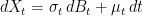
It is quite common to consider functions of real-time stochastic process which depend on whether or not it crosses a specified barrier level K. This can involve computing expectations involving a real-valued process X of the form

(1)

for a positive time T and function f: ℝ → ℝ. I am using the notation 𝔼[A;S] to denote the expectation of random variable A restricted to event S, or 𝔼[A1_S].

One example is computing prices of financial derivatives such as barrier options, where T represents the expiration time and f is the payoff at expiry conditional on hitting upper barrier level K. A knock-in call option would have the final payoff f(x) = (x - a)₊ for a contractual strike of a. Knock-out options are similar, except that the payoff is conditioned on not hitting the barrier level. As the sum of knock-in and knock-out options is just an option with no barrier, both cases involve similar calculations.

Alternatively, the barrier can be discrete, meaning that it only involves sampling the process at a finite set of times 0 ≤ t₁ ≤ ⋯ ≤ t_n ≤ T. Then, equation (1) is replaced by

(2)

Naturally, sampling at a finite set of times will reduce the probability of the barrier being reached and, so, if f is nonnegative then (2) will have a lower value than (1). It should still converge though as n goes to infinity and the sampling times become dense in the interval.

1. If the underlying process X is Brownian motion or geometric Brownian motion, possibly with a constant drift, then there are exact expressions for computing (1) in terms of integrating f against a normal density. See the post on the reflection principle for more information. However, it is difficult to find exact expressions for the discrete barrier (2) other than integrating over high-dimensional joint normal distributions. So, it can be useful to approximate a discrete barrier with analytic formulas for the continuous barrier. This is the idea used in the classic 1997 paper A Continuity Correction for Discrete Barrier Options by Broadie, Glasserman and Kou (freely available here).
2. We may want to compute the continuous barrier expectation (1) using Monte Carlo simulation. This is a common method, but involves generating sample paths of the process X at a finite set of times. This means that we are only able to sample at these times so, necessarily, are restricted to discrete barrier calculations as in (2).

I am primarily concerned with the second idea This is a very general issue, since Monte Carlo simulation is a common technique used in many applications. However, as it only represents sample paths at discrete time points, it necessarily involves discretely approximating continuous barrier levels. You may well ask why we would even want to use Monte Carlo if, as I mentioned above, there are exact expressions in these cases.In answer, such formulas only hold in very restrictive situations where the process X is a Brownian motion or geometric Brownian motion with constant drift. More generally it could be an ‘Ito process’ of the form

(3)

where B is standard Brownian motion. This describes X as a stochastic integral with respect to the predictable integrands σ and μ, which represent the volatility and drift of the process. Strictly speaking, these are ‘linear’ volatility and drift terms, rather than log-linear as used in many financial models applied to nonnegative processes such as stock prices. This is simply the choice made here, since this post is addressing a general mathematical problem of approximating continuous barriers and not restricting to such specific applications.

If the volatility and drift terms in (3) are not constant, then the exact formulas no longer hold. This is true, even if they are deterministic functions of time. In practice, these terms are often stochastic and can be rather general, in which case trying to find exact expressions is an almost hopeless task. Even though I concentrate on the case with constant volatility and drift in any calculations performed here, this is for convenience of exposition. The idea is that, as long as σ is piecewise continuous then, locally, it is well approximate as constant and the techniques discussed here should still apply.

In addition to considering general Ito processes (3), the ideas described here will apply to much more general functions of the process X than stated in (1). In the financial context, this means more general payoffs than simple knock-in or knock-out options. For example, autocallable trades involve a down-and-in put option but, additionally, contain a discrete set of upper barriers which cause the trade to make a final payment and terminate. They may also allow the issuer to early terminate the trade on a discrete set of dates. Furthermore, trades can depend on different assets with separate barriers on each of them, or on the average of a basket of assets, or have different barrier levels in different time periods. The list of possibilities is endless but, the idea is that each continuous barrier inside a complex payoff will be approximated by discretely sampled barrier conditions.

For efficiency, we may also want to approximate a discrete barrier with a large number of sampling times by one with fewer. The methods outlined in the post can also be used for this. In particular, the simple barrier shift described below could be used by taking the difference between the shift computed for the times actually sampled and the one for the required sample times. I do not go into details of this, but mention it now give an idea of the generality of the technique.

Let’s consider simply approximating a continuous barrier in (1) by the discrete barrier in (2). This will converge as the number of sampling times t_i increases but, the problem is, it converges very slowly. We can get an idea of the order of the error when the sampling times have a δt spacing which, with equally spaced times, is given by δt = T/n. This is as shown in figure 1 above. When the process first hits the continuous barrier level, it will be on average about δt/2 before the next sampling time. If X behaves approximately like a Brownian motion with volatiity σ over this interval then it will have about 50% chance of being above K at the next discrete time. On the other hand, it will be below K with about 50% probability, in which case with will drop a distance proportional to σ√δt below on average. This means that if the continuous barrier is hit, there is a probability roughly proportional to σ√δt that the discrete barrier is not hit. So, the error in approximating a continuous barrier (1) by the discrete case (2) is of the order of σ√δt which only tends to zero at rate 1/√n.

Figure 2 shows the result of computing the probability of hitting a continuous barrier minus the probability for a discrete one as a function of the number of sampling times n. This plot uses a standard Brownian motion so that σ = 1 and a terminal time T = 1, giving a barrier spacing of δt = 1/n. The level was set to K = 66% which has about 50% chance of being hit. The red line shows the difference computed using Monte Carlo simulation with 1 million paths, so that the numerical error is small enough to be comparable with the line thickness. The black line is proportional to 1/√n and, as indicated by the argument above, is a good approximation to the rate of convergence.

Such a slow rate of convergence is likely to necessitate having a very large number of sampling times in the Monte Carlo paths, which would be very inefficient.

---

Exact Expressions

One method of correcting the effect of using discrete sampling is to exactly simulate the maximum value across each time interval conditioned on the sampled values of the process. Suppose that X is Brownian motion with volatility σ > 0 and drift μ, so that it can be written as X₀ + σB_t + μt for standard Brownian motion B. Then, its maximum value X^∗_s,t ≡ sup_s≤u≤tX_u across interval [s, t] conditioned on its values at the ends of the interval is distributed according to

(4)

See theorem 3 of the post on the reflection principle and the comments thereafter, showing that this formula holds generally for Brownian motion with drift, so long as K ≥ X_s ∨ X_t. Using the fact that a random variable with cumulative distribution function F can be simulated as F^-1(U) for U uniformly distributed on the unit interval, (4) can be inverted to obtain

Using this to simulate the maximum of X between sampling times, we obtain the following exact expression for computing the barrier expectation.

Theorem 1 Let X be Brownian motion with volatility σ > 0 and drift μ. For times 0 = t₀ < t₁ < ⋯< t_n = T, let U₁, …, U_n be independent U(0, 1) random variables independent of X. Setting

Then

for all barrier levels K and measurable functions f such that f(X_T) is integrable.

So, if Monte Carlo simulation is used to sample the process at a set of discrete times, by generating additional random variables M_i as above, the continuous barrier expectation can be computed in the same way as for the discrete version (2) by replacing the X_ti with M_i in the barrier condition.

Alternatively, instead of simulating the additional random variables M_i, we can directly compute the probability (4) of hitting the continuous barrier conditional on the sampled values,

(5)

If the process does not reach the barrier level at any of the sample times, then it will have probability p_i of hitting it between times t_i-1 and t_i. So, the probability of not hitting in this interval is 1 – p_i and, by independence, these can be multiplied together to obtain the probability of not hitting the barrier conditioned on the sampled values. This gives the following alternative method.

Theorem 2 Let X be Brownian motion with volatility σ > 0 and drift μ. For times 0 = t₀ < t₁ < ⋯< t_n = T, define p_i by (5), which are functions of (X_ti-1, X_ti) and set

Then

for all barrier levels K and measurable functions f such that f(X_T) is integrable.

In fact, the expression in theorem 2 was used for the continuous barrier probability when computing the discretization errors in figure 2, even though it can be computed analytically. This is because, when taking the difference with the discrete barrier value it reduces the variance, so reducing Monte Carlo noise.

As discussed above, just handling Brownian motion with constant volatility and drift is rather restrictive. More generally, X can be an Ito process with time dependent volatility and drift. In this case, theorems 1 and 2 can still be applied as approximations. The only difference is that the constant volatility σ is replaced by the time-dependent one sampled at each interval. In the expressions for M_i and p_i, we replace σ by the sampled volatility σ̅_i at that time. Ideally, an average across the interval is used,

although the values of σ_u at times t_i-1 or t_i can also be used. So long as the volatility and drift has piecewise continuous paths, this approximation is good when the sampling times are dense. Across small time intervals, the volatility and drift will be close to constant. The result is that, although the methods given by theorems 1 and 2 are not exact, they will converge faster then rate 1/√n that was seen for naively approximating by the unadjusted discrete barrier.

---

Shifted Barrier Approximation

While the expressions above allow us to exactly correct for the discretization effect of sampling at a finite set of times, there are some practical issues with implementation. Supposing that we have already run a Monte Carlo simulation and generated samples of the process at a discrete set of times, the method described by theorem 1 would require going back and generating a new set of random numbers for each Monte Carlo path. This could be inconvenient if we are trying to modify an existing simulation, or if we are using a generic Monte Carlo simulation where it is not known at simulation time whether or not the minimum or maximum of the process will be needed. The method described by theorem 2 does not require simulating additional random variables. However, it does involve significantly modifying the function for which the expectation is required by adding additional terms involving the conditional expectation term q(X). This could get more complicated when applying to much more general ‘payoff’ functions, and is difficult to do in a very generic way.

Now I will look at a method which is not exact, but can be done by a very simple modification to the payoff function or by a simple shift to the sampled values of the process. The idea is similar to that described in the 1997 paper A Continuity Correction for Discrete Barrier Options by Broadie, Glasserman and Kou, and by the 2003 paper On Pricing of Discrete Barrier Options by Steven Kou. The motivation here is different though. Whereas they consider approximating a discrete barrier option in the Black-Scholes model by a continuous one, for which analytic solutions exist, we are considering approximating a continuous barrier by a discrete one for the purposes of Monte Carlo simulation.

When the process first reaches K at one of the discrete sampling times it will, in fact, be strictly above the level. If we let τ be the first time t_i at which the process is equal to or greater than K then the amount that it exceeds the level is the overshoot or excess R = X_τ – K. See figure 3. This overshoot effectively moves the barrier level up by distance R so that, to a leading order approximation, a discrete barrier at K is similar to a continuous barrier at level K + 𝔼[R]. So, we can compensate for this by shifting the discrete barrier level down by this amount.

By sequential analysis, the overshoot can be described in the limit as the sampling width δt goes to zero.

Theorem 3 Let X be Brownian motion with constant volatility σ > 0 and drift μ, and K > X₀ be a fixed level. For sampling width δt > 0, let

be the hitting time of the discrete barrier and R = X_τ – K be the overshoot. As δt tends to zero, the normalized excess R/(σ√δt) converges to a limiting distribution on [0, ∞) independent of X. This distribution does not depend on σ, μ, K and has mean

Before applying this, some explanations are in order. Convergence of the normalized excess refers to convergence in distribution to a limit μ. The independence from X is asymptotic. That is, for any bounded continuous function f: [0, ∞) → ℝ and any bounded random variable Z on the original probability space then, in the limit as the sampling width δt tends to zero,

So, in the limit of small δt, the normalised excess is approximated by a random variable of distribution μ independent of any fixed random variable Z. To be strict, for negative drift where there is a possibility that X never hits K, so the excess is undefined, we should condition these expectations on the barrier level being reached.

For a proof of the theorem 3, see lemma 10.11 of Siegmund, Sequential Analysis: Tests and Confidence Intervals. The stated value of β was computed in the 1965 paper, Sequential tests for the mean of a normal distribution IV by Chernoff. It is interesting that it involve the Riemann zeta function ζ, although maybe it is not so surprising. As per my previous post Brownian Motion and the Riemann Zeta Function, there are many such connections.

As explained above, discrete sampling effectively pushes the continuous barrier up by the random amount R. So, by asymptotic independence, the continuous barrier is shifted by an amount roughly independent of X. This shift can be approximated by its average value 𝔼[R] ≈ βσ√δt. To compensate for this, the discrete barrier level should be shifted down by the same amount.

Conjecture 4 Let X be Brownian motion with constant volatility σ > 0 and drift μ,. For fixed positive time T and integer n, consider the sampling width δt = T/n and times t_i = iδt. Then, for positive barrier K > X₀ define the shifted level

We have

as n → ∞ for any sufficiently regular function f: ℝ → ℝ.

I label this important result as a conjecture rather than a theorem, since finding exactly what ‘sufficiently regular’ means for f is not easy, and I do not include a proof. Siegmund-Yuh (1982), Brownian approximations for first passage probabilities, proves the result for f(X) of the form 1_{X<x} and, so, the conjecture does hold for piecewise constant functions.

The cases of knock-in call and put options are handled by Broadie, Glasserman and Kou (1997), A Continuity Correction for Discrete Barrier Options, and Kou (2003), On Pricing of Discrete Barrier Options. It seems that these methods extend to piecewise differentiable functions, although the regularity requirements for f can likely be relaxed further.

Conjecture 4 is saying that, by applying the shifted discrete barrier, a rate of convergence is obtained which is strictly better the O(1/√n) seen for the unshifted case. It does not, however, say how much faster the convergence is.

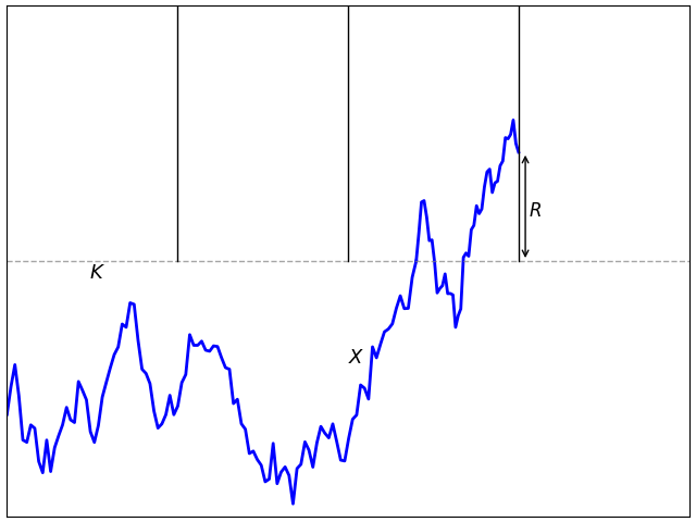
I repeated the experiment shown in figure 2, plotting the difference between the probability of hitting a continuous barrier and that of hitting a discrete barrier. As before, I use 1 million Monte Carlo simulations so that the noise is within the line width of the plot, a volatility of 1, so that it is standard Brownian motion, a terminal time T = 1, and barrier level K = 66%.. The difference between the continuous barrier probability and the discrete one is shown, both for the original barrier level of K and for the discrete shifted level of K – β√δt. The results are in figure 4 below, which shows that the shifted barrier level results in a much smaller error, and faster convergence as the number of sampling times increases.

Figure 5 below is scaled to better show the error using the shifted barrier approximation. Due to the smaller differences and scaling, this was calculated using 10 million Monte Carlo paths to further reduce the standard deviation. While some noise is still visible, it is not much more than a couple of line widths. We see that the error now scales like 1/n, which is much faster than the naive 1/√n seen above.

An advantage of using the barrier shift described here over the exact adjustments given further up, is that it is very simple. Suppose that we have already written a program to compute the barrier expectation in (2). No significant change to this is required to adjust for discreteness in sampling times. Only the barrier level passed to the program needs to be shifted.

Another way of expressing conjecture 4 is to consider shifting the process X up by the expected overshoot, rather than shifting the barrier level down. This gives the same criterion for hitting the barrier, but looking at it this way round has some advantages. Setting

(6)

the condition for hitting the barrier (2) becomes

The value M_i can be viewed as a proxy for the maximum of the process over time interval (t_i-1, t_i).

Using (6) to shift the samples of X has benefits over shifting the barrier level K. For one, it works even if the sampling times are not equally spaced. All that we have to do is to let δt represent the gap between successive sampling times t_i-1 and t_i, giving a time-dependent shift. It can also be applied for general Ito processes dX_t = σ_t dB_t + μ_t dt with stochastic volatility and drift. The only change is that σ is replaced by an average of the volatility across the time step, as for the exact methods further above. This is a stochastic shift, but is no problem so long as the volatility is positive and piecewise continuous, and hence can be locally approximated by constant volatility. Then (6) should still give better convergence than the O(1/√n) seen with the naive sampling of (2).

As a final note, the adjustments described above all involve knowing the volatility of the process. It can be desirable to remove this to obtain adjustments which are model independent. They can then be tacked onto any simulation without requiring it to explicitly generate samples for the volatility paths. I will look at this idea more in a future post.