Normal Maps

Given two *-probability spaces ${(\mathcal A,p)}$ and ${(\mathcal A^\prime,p^\prime)}$ , we want to consider maps ${\varphi\colon\mathcal A\rightarrow\mathcal A^\prime}$ . For example, we can look homomorphisms, which preserve the *-algebra operations, and can also consider restricting to state-preserving maps satisfying ${p^\prime(\varphi(a))=p(a)}$ . In algebraic probability theory, however, it is often necessary to include a continuity condition, leading to the idea of normal maps, which I look at in this post. In fact, as we will see, all *-homomorphisms between commutative probability spaces which preserve the state are normal, so this concept is most important in the noncommutative setting.

In contrast to the previous few posts on algebraic probability, the current post is a bit of a gear-change. We are still concerned with with the basic concepts of *-algebras and states. However, the main theorem stated below, which reduces to the Radon-Nikodym theorem in the commutative case, is deeper and much more difficult to prove than the relatively simple results with which I have been concerned with so far.

The weak topology on a *-probability space ${(\mathcal A,p)}$ is the weakest topology making the maps

$\displaystyle \setlength\arraycolsep{2pt} \begin{array}{rl} &\displaystyle \mathcal A\rightarrow{\mathbb C},\smallskip\\ &\displaystyle a\mapsto p(xay), \end{array}$

continuous, for all ${x,y\in\mathcal A}$ . This definition means that a net ${a_\alpha\in\mathcal A}$ converges to a limit ${a}$ in the weak topology if and only if ${p(xa_\alpha y)\rightarrow p(xay)}$ for all ${x,y\in\mathcal A}$ . In fact, the weak topology on the whole of ${\mathcal A}$ can be a bit too weak, so we will restrict to bounded sets. The ${L^\infty}$ seminorm is defined on any *-probability space ${(\mathcal A,p)}$ , and elements ${a\in\mathcal A}$ are said to be bounded if ${\lVert a\rVert_\infty}$ is finite. The unit ball in ${\mathcal A}$ with respect to this seminorm is,

$\displaystyle \mathcal A_1=\left\{a\in\mathcal A\colon\lVert a\rVert_\infty\le1\right\}.$

I will only define normal maps for bounded *-probability spaces and, although the notion of normality can be extended to more general linear maps, I concentrate on homomorphisms in this post. We say that ${(\mathcal A,p)}$ is bounded if every ${a\in\mathcal A}$ is bounded.

Definition 1 Let ${(\mathcal A,p)}$ and ${(\mathcal A^\prime,p^\prime)}$ be bounded *-probability spaces. Then, a *-homomorphism ${\varphi\colon\mathcal A\rightarrow\mathcal A^\prime}$ is normal iff it is weakly continuous on ${\mathcal A_1}$ .

We previously showed that, in many cases, homomorphisms between *-probability spaces are ${L^\infty}$ -continuous. This also holds for normal maps.

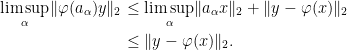
Lemma 2 Let ${(\mathcal A,p)}$ and ${(\mathcal A^\prime,p^\prime)}$ be bounded *-probability spaces and ${\varphi\colon\mathcal A\rightarrow\mathcal A^\prime}$ be a normal *-homomorphism. Then, ${\varphi}$ is ${L^\infty}$ -isometric, so that ${\lVert\varphi(a)\rVert_\infty=\lVert a\rVert_\infty}$ for all ${a\in\mathcal A}$ . In particular,

$\displaystyle \varphi(\mathcal A_1)\subseteq\mathcal A^\prime_1.$ (1)

Proof: By lemma 2 of the post on homomorphisms, it is sufficient to show that (1) holds. Suppose, on the contrary, that this is false. Then, there exists ${a\in\mathcal A}$ such that ${\lVert a\rVert < 1}$ , but ${\lVert\varphi(a)\rVert > 1}$ . So,

$\displaystyle \lVert (a^*a)^n\rVert=\lVert a\rVert^{2n}\rightarrow0$

as ${n\rightarrow\infty}$ . So, ${(a^*a)^n\rightarrow0}$ in the ${L^\infty(p)}$ topology and, hence, also in the weak topology. Then, there exists ${x\in\mathcal A^\prime}$ such that ${\lVert x\rVert_2\le1}$ and ${\lVert \varphi(a)x\rVert_2 > 1}$ . As

$\displaystyle p^\prime(x^*\varphi((a^*a)^n)x)^{\frac1{2n}}= p^\prime(x^*(\varphi(a)^*\varphi(a))^nx)^{\frac1{2n}}$

is increasing in ${n}$ ,

$\displaystyle p^\prime(x^*\varphi((a^*a)^n)x)\ge1$

does not tend to zero, contradicting weak continuity. ⬜

A consequence of this is that compositions of normal maps are normal. That is, if ${f}$ and ${g}$ are normal homomorphisms ${\mathcal A\rightarrow\mathcal A^\prime}$ and, respectively, ${\mathcal A^\prime\rightarrow\mathcal A^{\prime\prime}}$ , then the composition ${g\circ f}$ between ${\mathcal A}$ and ${\mathcal A^{\prime\prime}}$ is also normal. This follows from the fact that compositions of continuous maps are continuous.

Corollary 3 Compositions of normal homomorphisms are normal.

Normal homomorphisms have various characterisations. For example, we will show the following result (see theorem 8 below), which is related to the existence of conditional expectations in classical probability theory.

Theorem 4 Let ${(\mathcal A,p)}$ and ${(\mathcal A^\prime,p^\prime)}$ be bounded *-probability spaces. Then, a *-homomorphism ${\varphi\colon\mathcal A\rightarrow\mathcal A^\prime}$ is normal if and only if, for every ${x,y\in\mathcal A^\prime}$ , there exists sequences ${x_n,y_n\in\mathcal A}$ satisfying

$\displaystyle \sum_{n=1}^\infty p(x_n^*x_n+y_n^*y_n) < \infty,$ (2)

such that

$\displaystyle p^\prime(x^*\varphi(a)y)=\sum_{n=1}^\infty p(x_n^*ay_n)$ (3)

for all ${a\in\mathcal A}$ .

Note that condition (2) is sufficient for the sum (3) to be absolutely convergent.

$\displaystyle \setlength\arraycolsep{2pt} \begin{array}{rl} \displaystyle \sum_{n=1}^\infty \lvert p(x_n^*ay_n)\rvert&\displaystyle\le\lVert a\rVert\sum_n\sqrt{p(x_n^*x_n)p(y_n^*y_n)}\smallskip\\ &\displaystyle\le\frac12\lVert a\rVert\sum_n p(x_n^*x_n+y_n^*y_n). \end{array}$

Before going into detail on normal homomorphisms, we note that the concept applies more generally than just for *-probability spaces. In fact, normal maps are usually studied in the context of von Neumann algebras. In order to include such generalisations, I will not restrict solely to *-probability spaces below. As in the previous post, we call a pair ${(\mathcal A,V)}$ a *-algebra representation, where ${\mathcal A}$ is a *-algebra, ${V}$ is a semi-inner product space, and ${\mathcal A}$ acts on ${V}$ by left multiplication. The operator seminorm on ${\mathcal A}$ is denoted by ${\lVert\cdot\rVert}$ , and the representation will be called bounded if ${\lVert a\rVert}$ is finite for all ${a\in\mathcal A}$ . 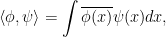As previously, ${V^\infty}$ denotes the sequences ${x=(x_n)}$ in ${V}$ such that ${\sum_n\lVert x_n\rVert^2}$ is finite, which has the semi-inner product ${\langle x,y\rangle=\sum_n\langle x_n,y_n\rangle}$ . An element ${a\in\mathcal A}$ acts diagonally on ${V^\infty}$ by ${ax=(ax_n)}$ , so that ${(\mathcal A,V^\infty)}$ is a *-algebra representation.

A *-probability space ${(\mathcal A,p)}$ defines a *-algebra representation ${(\mathcal A,\mathcal A)}$ with semi-inner product ${\langle x,y\rangle=p(x^*y)}$ and with ${\mathcal A}$ acting on itself by left-multiplication.

The Main Theorem

The following result, applying to linear functionals on ${\mathcal A}$ , is the main result of this post. A linear map ${F\colon\mathcal A\rightarrow{\mathbb C}}$ is called normal if it satisfies the equivalent conditions of theorem 5. This relates the weak, strong, ultraweak and ultrastrong operator topologies.

Theorem 5 Let ${(\mathcal A,V)}$ be a bounded *-algebra representation, and ${F\colon\mathcal A\rightarrow{\mathbb C}}$ be a linear function. Then, the following are equivalent.

${F}$ is weakly continuous on ${\mathcal A_1}$ .

${F}$ is strongly continuous on ${\mathcal A_1}$ .

${F}$ is ultraweakly continuous.

${F}$ is ultrastrongly continuous.

There exists ${x,y\in V^\infty}$ such that ${F(a)=\langle x,ay\rangle}$ for all ${a\in\mathcal A}$ .

Proof: The implications 1 ⇒ 2 and 3 ⇒ 4 follow immediately from the fact that the strong and ultrastrong topologies are stronger than the weak and ultraweak topologies respectively. The implications 3 ⇒ 1 and 4 ⇒ 1 follow from lemma 7 of the operator topology post. The implication 5 ⇒ 3 is immediate from the definition of the ultraweak topology.

The result now follows once we establish the implication 2 ⇒ 5. However, this is by far the most involved part of the theorem, so the proof is left until later. ⬜

It is important to note that, for a bounded *-probability space, the state is always normal. This is an immediate consequence of lemma 10 of the operator topology post.

Lemma 6 Let ${(\mathcal A,p)}$ be a bounded *-probability space. Then, ${p}$ is normal.

For classical probability spaces, theorem 5 is effectively the Radon-Nikodym theorem.

Lemma 7 Let ${(\Omega,\mathcal F,{\mathbb P})}$ be a probability space. With respect to the *-probability space ${(L^\infty(\Omega,\mathcal F,{\mathbb P}),{\mathbb P})}$ , the following are equivalent for any linear map ${F\colon L^\infty\rightarrow{\mathbb C}}$ ,

${F}$ is continuous in probability on the unit ball of ${L^\infty}$ .

${F(A)={\mathbb E}[AZ]}$ for some ${Z\in L^1}$ .

${F}$ is normal.

Proof: The result follows from theorem 5 since, by lemma 12 of the operator topology post, the first statement of the lemma is equivalent to statement 2 of the theorem the second is equivalent to statement 5 of the theorem. ⬜

Normal Homomorphisms

Applying theorem 5 to homomorphisms between algebras gives the result below, and any *-homomorphism satisfying the equivalent conditions is called normal. I note that theorem 4 is a consequence of the equivalence between statements 1 and 5.

Theorem 8 Let ${(\mathcal A,V)}$ and ${(\mathcal A^\prime,V^\prime)}$ be bounded *-algebra representations, and ${\varphi\colon\mathcal A\rightarrow\mathcal A^\prime}$ be a *-homomorphism. Then, the following are equivalent.

${\varphi}$ is weakly continuous on ${\mathcal A_1}$ .

${\varphi}$ is strongly continuous on ${\mathcal A_1}$ .

${\varphi}$ is ultraweakly continuous.

${\varphi}$ is ultrastrongly continuous.

${F\circ\varphi}$ is normal for all normal linear maps ${F\colon\mathcal A^\prime\rightarrow{\mathbb C}}$ .

Furthermore, if these conditions hold then ${\varphi}$ is norm-bounded such that ${\lVert\varphi(a)\rVert\le\lVert a\rVert}$ for all ${a\in\mathcal A}$ or, equivalently, ${\varphi(\mathcal A_1)\subseteq\mathcal A^\prime_1}$ .

Proof: 1 ⇒ 2: If ${a_\alpha\in\mathcal A_1}$ tends to strongly to zero, then ${a_\alpha^*a_\alpha\in\mathcal A_1}$ tends weakly to zero, by lemma 2 on operator topologies. Hence, ${\varphi(a_\alpha)^*\varphi(a_\alpha)=\varphi(a_\alpha^*a_\alpha)}$ tends weakly to zero and, again by lemma 2, ${\varphi(a_\alpha)\rightarrow0}$ strongly.

3 ⇒ 4: If ${a_\alpha\in\mathcal A}$ tends to zero ultrastrongly then ${a_\alpha^*a_\alpha\rightarrow0}$ ultraweakly, by lemma 5 on operator topologies. Hence, ${\varphi(a_\alpha)^*\varphi(a_\alpha)=\varphi(a_\alpha^*a_\alpha)}$ tends ultraweakly to zero and, again by lemma 5, ${\varphi(a_\alpha)\rightarrow0}$ ultrastrongly.

3 ⇒ 1: By lemma 9 on operator topologies, the weak and ultraweak topologies coincide on ${\mathcal A_1}$ , so ${\varphi}$ is continuous with respect to the weak topology on ${\mathcal A_1}$ and the ultraweak topology on ${\mathcal A^\prime}$ . As the ultraweak topology is stronger than the weak topology, this means that ${\varphi}$ is continuous with respect to the weak topologies on ${\mathcal A_1}$ and ${\mathcal A^\prime}$ .

4 ⇒ 2: By lemma 9 on operator topologies, the strong and ultrastrong topologies coincide on ${\mathcal A_1}$ , so ${\varphi}$ is continuous with respect to the strong topology on ${\mathcal A_1}$ and the ultrastrong topology on ${\mathcal A^\prime}$ . As the ultrastrong topology is stronger than the strong topology, this means that ${\varphi}$ is continuous with respect to the strong topologies on ${\mathcal A_1}$ and ${\mathcal A^\prime}$ .

5 ⇒ 3: Let ${a_\alpha\in\mathcal A}$ be a net tending ultraweakly to zero. Then, for any normal linear map ${F\colon\mathcal A^\prime\rightarrow{\mathbb C}}$ , ${F\circ\varphi}$ is normal. Hence, ${F(\varphi(a_\alpha))}$ tends to zero, showing that ${\varphi(a_\alpha)\rightarrow0}$ ultraweakly.

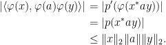
2 ⇒ 5: Let us first show that ${\varphi(\mathcal A_1)\subseteq\mathcal A^\prime_1}$ . If not, then there exists ${a\in\mathcal A}$ with ${\lVert a\rVert < 1}$ and ${\lVert\varphi(a)\rVert > 1}$ . Then, ${\lVert (a^*a)^n\rVert=\lVert a\rVert^{2n}\rightarrow0}$ as ${n\rightarrow\infty}$ . In particular, ${(a^*a)^n\rightarrow0}$ strongly. Setting ${b=\varphi(a)}$ , choose ${\xi\in V^\prime}$ with ${\lVert\xi\rVert\le 1}$ and ${\lVert b\xi\rVert > 1}$ . Also, define ${p\colon\mathcal A^\prime\rightarrow{\mathbb C}}$ by ${p(c)=\langle\xi,c\xi\rangle}$ . This is a positive linear map satisfying ${\lVert p\rVert\le1}$ . Hence, by lemma 7 of the post on states, ${p((b^*b)^n)^{\frac1{2n}}}$ is increasing in ${n}$ . So,

$\displaystyle \setlength\arraycolsep{2pt} \begin{array}{rl} \displaystyle \langle\xi,\varphi((a^*a)^n)\xi\rangle&\displaystyle=\langle\xi,(b^*b)^n\xi\rangle=p((b^*b)^n)\smallskip\\ &\displaystyle\ge p(b^*b)^{n}=\lVert b\xi\rVert^{2n}\ge1, \end{array}$

contradicting the condition that ${\varphi((a^*a)^n)\rightarrow0}$ strongly. Hence, ${\varphi(\mathcal A_1)\subseteq\mathcal A^\prime_1}$ as required.

Now, suppose that ${F\colon\mathcal A^\prime\rightarrow{\mathbb C}}$ is a normal linear map. Then, ${F}$ is strongly continuous on ${\mathcal A^\prime_1}$ and, hence, ${F\circ\varphi}$ is strongly continuous on ${\mathcal A_1}$ , so is normal. ⬜

Recall that a homomorphism of *-probability spaces ${(\mathcal A,p)}$ and ${(\mathcal A^\prime,p^\prime)}$ is a *-homomorphism ${\varphi\colon\mathcal A\rightarrow\mathcal A^\prime}$ preserving the state, ${p^\prime(\varphi(a))=p(a)}$ . Any such map is automatically an ${L^2}$ -isometry,

$\displaystyle \setlength\arraycolsep{2pt} \begin{array}{rl} \displaystyle \langle\varphi(x),\varphi(y)\rangle &\displaystyle = p^\prime\left(\varphi(x)^*\varphi(y)\right)\smallskip\\ &\displaystyle=p^\prime\left(\varphi(x^*y)\right)\smallskip\\ &\displaystyle=p(x^*y)=\langle x,y\rangle. \end{array}$

For commutative *-algebras, this is sufficient to imply that that it is normal. More generally, it is enough to know that ${p^\prime}$ is tracial so that ${p^\prime(ab)=p^\prime(ba)}$ for all ${a,b\in\mathcal A^\prime}$ .

Lemma 9 Let ${\varphi}$ be a homomorphism between bounded *-probability spaces ${(\mathcal A,p)}$ and ${(\mathcal A^\prime,p^\prime)}$ . If ${\mathcal A^\prime}$ is commutative or, more generally, if ${p^\prime}$ is tracial, then ${\varphi}$ is normal.

Proof: As explained above, we know that ${\varphi}$ is ${L^2}$ -continuous. However, the strong topology coincides with ultrastrong on ${\mathcal A_1}$ , which is stronger then ${L^2}$ convergence and, as ${p^\prime}$ is tracial, ${L^2}$ convergence is stronger than strong convergence on ${\mathcal A^\prime}$ . So, ${\varphi}$ is strongly continuous on ${\mathcal A_1}$ and, by theorem 8, is normal. ⬜

For noncommutative algebras, and non-tracial states, homomorphisms of *-probability spaces need not be normal. The following result can be useful, in some situations, to ensure normality.

Lemma 10 Let ${(\mathcal A,p)}$ and ${(\mathcal A^\prime,p^\prime)}$ be bounded *-probability spaces and ${\varphi\colon\mathcal A\rightarrow\mathcal A^\prime}$ be a *-homomorphism. Each of the following statements implies the next one:

${\varphi(\mathcal A)}$ is ultrastrongly dense in ${\mathcal A^\prime}$ ,

${\varphi(\mathcal A)}$ is ${L^2}$ -dense in ${\mathcal A^\prime}$ ,

and, if ${\varphi}$ preserves the state,

${\varphi}$ is normal.

Proof: 1 ⇒ 2: By lemma 11 on operator topologies, the ultrastrong topology is stronger than the ${L^2}$ topology, so ${\varphi(\mathcal A)}$ is ${L^2}$ -dense in ${\mathcal A}$ .

2 ⇒ 3: For any ${a,x,y\in\mathcal A}$ then, if ${\varphi}$ preserves the state,

$\displaystyle \setlength\arraycolsep{2pt} \begin{array}{rl} \displaystyle \lvert\langle\varphi(x),\varphi(a)\varphi(y)\rangle\rvert&\displaystyle=\lvert p^\prime(\varphi(x^*ay))\rvert\smallskip\\ &\displaystyle=\lvert p(x^*ay)\rvert\smallskip\\ &\displaystyle\le\lVert x\rVert_2\lVert a\rVert\lVert y\rVert_2. \end{array}$

As ${\varphi(\mathcal A)}$ is ${L^2}$ -dense in ${\mathcal A^\prime}$ ,

$\displaystyle \lvert\langle x,\varphi(a)y\rangle\rvert\le\lVert x\rVert_2\lVert a\rVert\lVert y\rVert_2$

for all ${x,y\in\mathcal A^\prime}$ and, hence, ${\lVert\varphi(a)\rVert\le\lVert a\rVert}$ .

Now suppose that ${a_\alpha\in\mathcal A_1}$ tends strongly zero. Then, for any ${x\in\mathcal A}$ and ${y\in\mathcal A^\prime}$ ,

$\displaystyle \lVert\varphi(a_\alpha) y\rVert_2\le\lVert\varphi(a_\alpha x)\rVert_2+\lVert\varphi(a_\alpha)\rVert\lVert y-\varphi(x)\rVert_2$

so, taking the limit,

$\displaystyle \setlength\arraycolsep{2pt} \begin{array}{rl} \displaystyle \limsup_\alpha\lVert \varphi(a_\alpha) y\rVert_2&\displaystyle\le\limsup_\alpha\lVert a_\alpha x\rVert_2+\lVert y-\varphi(x)\rVert_2\smallskip\\ &\displaystyle\le\lVert y-\varphi(x)\rVert_2. \end{array}$

As ${\varphi(\mathcal A)}$ is ${L^2}$ -dense in ${\mathcal A^\prime}$ , ${x}$ can be chosen to make the right-hand-side as small as we like and, hence, ${\varphi(a_\alpha)\rightarrow0}$ strongly. So, ${\varphi}$ is normal. ⬜

As an example of theorem 8 applied to classical probability spaces, it immediately implies the existence of conditional expectations.

Corollary 11 Let ${(\Omega,\mathcal F,{\mathbb P})}$ be a probability space and ${\mathcal G}$ be a sub-sigma-algebra of ${\mathcal F}$ . Then, for any ${Z\in L^1(\Omega,\mathcal F,{\mathbb P})}$ , there exists ${Y\in L^1(\Omega,\mathcal G,{\mathbb P})}$ satisfying ${{\mathbb E}[XY]={\mathbb E}[XZ]}$ for all ${X\in L^\infty(\Omega,\mathcal G,{\mathbb P})}$ .

Proof: Let ${\mathcal A=L^\infty(\Omega,\mathcal G,{\mathbb P})}$ , ${\mathcal A^\prime=L^\infty(\Omega,\mathcal F,{\mathbb P})}$ , and ${\varphi\colon\mathcal A\rightarrow\mathcal A^\prime}$ be the inclusion map. As ${\mathcal A^\prime}$ is commutative, lemma 9 says that ${\varphi}$ is normal. Now, for any ${Z\in L^1(\Omega,\mathcal F,{\mathbb P})}$ , lemma 12 of the operator topology post applies, so that ${F(A)={\mathbb E}[AZ]}$ is a normal map on ${\mathcal A^\prime}$ and, by theorem 8 above, ${F\circ\varphi}$ is normal. Applying lemma 12 on operator topologies another time, there exists ${Y\in L^1(\Omega,\mathcal G,{\mathbb P})}$ satisfying

$\displaystyle {\mathbb E}[XZ]=F\circ\varphi(X)={\mathbb E}[XY]$

for all ${X\in\mathcal A}$ . ⬜

Finally, I note that homomorphisms of *-probability spaces are not always normal. Example 2 of the post on homomorphisms gives an example of a homomorphism ${\varphi}$ which is not ${L^\infty}$ -continuous, so cannot be normal. However, even if ${\varphi}$ is ${L^\infty}$ -continuous, it need not be normal.

Example 1 An ${L^\infty}$ -continuous homomorphism ${\varphi}$ between bounded *-probability spaces ${(\mathcal A,p)}$ and ${(\mathcal A^\prime,p^\prime)}$ which is not normal.

In this example, let ${\mathcal H=L^2({\mathbb R})}$ be the Hilbert space of square-integrable functions ${{\mathbb R}\rightarrow{\mathbb C}}$ with inner product

$\displaystyle \langle\phi,\psi\rangle=\int\overline{\phi(x)}\psi(x)dx,$

and let ${\mathcal A^\prime=B(\mathcal H)}$ be the *-algebra of bounded linear maps ${\mathcal H\rightarrow\mathcal H}$ . If ${\xi=1_{[0,1]}\in\mathcal H}$ , then we define the state

$\displaystyle p^\prime(a)=\langle\xi,a\xi\rangle$

on ${\mathcal A^\prime}$ . For bounded measurable ${f\colon{\mathbb R}\rightarrow{\mathbb C}}$ , define ${M_f\in\mathcal A^\prime}$ to be multiplication by ${f}$ , ${M_f\psi(x)=f(x)\psi(x)}$ . Let ${\mathcal A}$ be the subalgebra of ${\mathcal A^\prime}$ consisting of the elements ${M_f}$ for continuous functions ${f\colon{\mathbb R}\rightarrow{\mathbb C}}$ which are constant on each of the intervals ${(-\infty,0]}$ and ${[1,\infty)}$ . We then let ${p}$ be the restriction of ${p^\prime}$ to ${\mathcal A}$ , and ${\varphi\colon\mathcal A\rightarrow\mathcal A^\prime}$ be inclusion. This is clearly a homomorphism between the *-probability spaces ${(\mathcal A,p)}$ and ${(\mathcal A^\prime,p^\prime)}$ .

The ${L^\infty}$ -norm of ${M_f\in\mathcal A}$ with respect to ${(\mathcal A^\prime,p^\prime)}$ is the supremum of ${\lvert f\rvert}$ and, with respect to ${(\mathcal A,p)}$ it is the supremum on the unit interval. As ${f}$ is constant on the intervals ${(-\infty,0]}$ and ${[1,\infty)}$ , these are the same, so ${\varphi}$ is ${L^\infty}$ -isometric,

Next, consider ${f(x)=x}$ for ${0\le x\le1}$ , ${f(x)=0}$ for ${x\le0}$ , and ${f(x)=1}$ for ${x\ge1}$ . Then, ${M_f\in\mathcal A}$ and we compute,

$\displaystyle p(M_f^n)=\int_0^1x^ndx=\frac1n\rightarrow0.$

As ${\mathcal A}$ is commutative, this says that ${M_f^n\rightarrow0}$ strongly in ${(\mathcal A,p)}$ . However, the unitary ${U\in\mathcal A^\prime}$ defined by ${U\psi(x)=\psi(x-1)}$ satisfies ${U^*M_fU=M_g}$ , where ${g(x)=f(x+1)}$ is equal to ${1}$ on the unit interval. Hence,

$\displaystyle p^\prime(U^*M_f^nU)=1$

for all ${n}$ , showing that ${M_f^n}$ does not tend weakly or strongly to zero in ${(\mathcal A^\prime,p^\prime)}$ . So, ${\varphi}$ is not normal.

Proof of Theorem 5

Throughout this section, I take ${(\mathcal A,V)}$ to be a bounded *-algebra representation, and use ${\lVert a\rVert}$ to denote the operator norm of ${a\in\mathcal A}$ . For any any ${x,y\in V^\infty}$ , define the linear map

$\displaystyle \setlength\arraycolsep{2pt} \begin{array}{rl} &\displaystyle F_{x,y}\colon\mathcal A\rightarrow{\mathbb C},\smallskip\\ &\displaystyle F_{x,y}(a)=\langle x,ay\rangle. \end{array}$

(4)

Denote the space of all such linear maps by ${\mathcal A_*}$ . The remainder of this post is devoted to the following result, which will complete the proof of theorem 5.

Theorem 12 If ${F\colon\mathcal A\rightarrow{\mathbb C}}$ is a linear map and is strongly continuous on ${\mathcal A_1}$ , then ${F\in\mathcal A_*}$ .

This statement is, by far, the most mathematically involved result of this post, so we prove it step-by-step. It will also require a couple of powerful, but standard, theorems of operator algebras and functional analysis. Namely, we will rely on the Krein–Smulian and Kaplansky density theorems. As the Krein–Smulian theorem gives a condition for a linear functional on the dual of a Banach space to be weakly continuous, the method we will use to prove theorem 4 will start by showing that ${\mathcal A_*}$ is a Banach space and that the relevant completion of ${\mathcal A}$ is its Banach dual. The completion that we use will be the von Neumann algebra generated by ${\mathcal A}$ , although I will not make use of the theory of von Neumann algebras here.

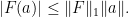
For now, note that the inequality

$\displaystyle \lvert F_{x,y}(a)\rvert=\lvert\langle x,ay\rangle\rvert\le\lVert x\rVert\lVert a\rVert\lVert y\rVert$

shows that every ${F_{x,y}\in\mathcal A_*}$ is bounded, with operator norm ${\lVert F_{x,y}\rVert\le\lVert x\rVert\lVert y\rVert}$ . As elements of ${\mathcal A_*}$ can be expressed in the form ${F_{x,y}}$ in many different ways, define a norm by taking the infimum over all such representations,

$\displaystyle \lVert F\rVert_1=\inf\left\{\lVert x\rVert\lVert y\rVert\colon x,y\in V^\infty,F=F_{x,y}\right\}.$

In particular, for ${F\in\mathcal A_*}$ and ${a\in\mathcal A}$ , the following inequality holds,

$\displaystyle \lvert F(a)\rvert\le\lVert F\rVert_1\lVert a\rVert.$

(5)

As yet, we have not even shown that ${\mathcal A_*}$ is closed under linear combinations, so is a vector space, nor have we shown that ${\lVert\cdot\rVert_1}$ is a norm. In fact, not only are these statements true, but ${\mathcal A_*}$ is a Banach space.

Lemma 13 ${\mathcal A_*}$ is a Banach space under the norm ${\lVert\cdot\rVert_1}$ .

Proof: We need to show that ${\mathcal A_*}$ is a vector space, and that ${\lVert\cdot\Vert_1}$ is a norm with respect to which ${\mathcal A_*}$ is complete.

Is is straightforward that ${\lVert\cdot\rVert_1}$ is positive definite since, if ${\lVert F\rVert_1=0}$ , then (5) gives ${F=0}$ . Now suppose that ${F\in\mathcal A_*}$ and ${\lambda\in{\mathbb C}}$ . Then, ${F=F_{x,y}}$ for some ${x,y\in V^\infty}$ . So, ${\lambda F=F_{x,\lambda y}}$ is in ${\mathcal A_*}$ and,

$\displaystyle \lVert\lambda F\rVert_1\le\lvert\lambda\rvert\lVert x\rVert\lVert y\rVert.$

Taking the infimum over all such ${x}$ and ${y}$ gives ${\lVert\lambda F\rVert_1\le\lvert\lambda\rvert\lVert F\rVert_1}$ .

Next, consider a sequence ${F_n\in\mathcal A_*}$ with ${\sum_n\lVert F_n\rVert_1}$ finite. Using the fact that

$\displaystyle \sum_n\lvert F_n(a)\rvert\le\sum_n \lVert F_n\rVert_1\lVert a\rVert < \infty,$

we can define ${F\colon\mathcal A\rightarrow{\mathbb C}}$ by the absolutely convergent sum

$\displaystyle F(a)=\sum_nF_n(a).$

We show that ${F}$ is in ${\mathcal A_*}$ .

Fixing ${\epsilon > 0}$ , choose ${x_n,y_n\in V^\infty}$ such that ${F_n=F_{x_n,y_n}}$ and ${\lVert x_n\rVert\lVert y_n\rVert\le\lVert F_n\rVert_1+2^{-n}\epsilon}$ . By scaling we can assume, without loss of generality, that ${\lVert x_n\rVert=\lVert y_n\rVert}$ . Decomposing ${x_n=(x_{nm})}$ and ${y_n=(y_{nm})}$ then,

$\displaystyle F_n(a)=\langle x_n,a y_n\rangle=\sum_{m=1}^\infty\langle x_{nm},ay_{nm}\rangle.$

Letting ${k\mapsto(n_k,m_k)}$ be a bijection from ${{\mathbb N}}$ to ${{\mathbb N}\times{\mathbb N}}$ then,

$\displaystyle F(a)=\sum_{m,n=1}^\infty\langle x_{nm},ay_{nm}\rangle=F_{x,y}(a)$

where we have defined ${x,y\in V^\infty}$ by ${x=(x_{n_km_k})}$ and ${y=(y_{n_km_k})}$ . So, ${F\in\mathcal A_*}$ and,

$\displaystyle \setlength\arraycolsep{2pt} \begin{array}{rl} &\displaystyle \lVert x\rVert^2=\sum_{m,n=1}^\infty\lVert x_{nm}\rVert^2=\sum_{n=1}^\infty\lVert x_n\rVert^2=\sum_{n=1}^\infty\lVert x_n\rVert\lVert y_n\rVert,\smallskip\\ &\displaystyle \lVert y\rVert^2=\sum_{m,n=1}^\infty\lVert y_{nm}\rVert^2=\sum_{n=1}^\infty\lVert y_n\rVert^2=\sum_{n=1}^\infty\lVert x_n\rVert\lVert y_n\rVert. \end{array}$

So,

$\displaystyle \lVert F\rVert_1\le\lVert x\rVert\lVert y\rVert\le\sum_{n=1}^\infty\lVert x_n\rVert\lVert y_n\rVert\le\sum_{n=1}^\infty\lVert F_n\rVert_1+\epsilon.$

As ${\epsilon}$ is arbitrary, we obtain

$\displaystyle \lVert F\rVert_1\le\sum_{n=1}^\infty\lVert F_n\rVert_1.$

(6)

In particular, for any ${F_1,F_2\in\mathcal A_*}$ , taking ${F_n=0}$ for ${n > 2}$ in the argument above shows that ${F\equiv F_1+F_2}$ is in ${\mathcal A_*}$ with ${\lVert F\rVert_1\le\lVert F_1\rVert_1+\lVert F_2\rVert_1}$ . Hence, ${\mathcal A_*}$ is a vector space and ${\lVert\cdot\rVert_1}$ is a norm.

It only remains to prove completeness. So, consider a Cauchy sequence ${F_n\in\mathcal A_*}$ . By (5), ${F_n(a)}$ is Cauchy for any ${a\in\mathcal A}$ and, hence, we can define ${F\colon\mathcal A\rightarrow{\mathbb C}}$ by ${F(a)=\lim_nF_n(a)}$ . Choosing a subsequence ${F_{n_k}}$ satisfying ${\lVert F_m-F_{n_k}\rVert_1\le2^{-k}}$ whenever ${m\ge n_k}$ , by the argument above and inequality (6), ${F-F_n}$ is in ${\mathcal A_*}$ with

$\displaystyle \setlength\arraycolsep{2pt} \begin{array}{rl} \displaystyle \lVert F-F_n\rVert_1&\displaystyle\le\lVert F_n-F_{n_j}\rVert_1+\sum_{k=j}^\infty\lVert F_{n_{k+1}}-F_{n_k}\rVert_1\smallskip\\ &\displaystyle\le\lVert F_n-F_{n_j}\rVert_1+\sum_{k=j}^\infty 2^{-k}\smallskip\\ &\displaystyle=\lVert F_n-F_{n_j}\rVert_1+2^{1-j}. \end{array}$

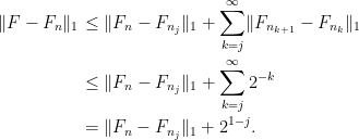
Letting ${j}$ increase to infinity,

$\displaystyle \lVert F-F_n\rVert_1\le\sup_{m\ge n}\lVert F_n-F_m\rVert_1\rightarrow0$

shows that ${F_n}$ is norm convergent to ${F}$ . ⬜

The following is a standard result for a *-algebra acting on a Hilbert space.

Lemma 14 Let ${(\mathcal A,\mathcal H)}$ be a bounded *-algebra representation, with ${\mathcal H}$ a Hilbert space. Then, for a linear map ${F\colon\mathcal A\rightarrow{\mathbb C}}$ , the following are equivalent:

${F}$ is weakly continuous.

${F}$ is strongly continuous.

There exists finite sequences ${x_k,y_k\in\mathcal H}$ ( ${k=1,\ldots,n}$ ) such that

$\displaystyle F(a)=\sum_{k=1}^n\langle x_n,ay_n\rangle.$ (7)

Proof: 1 ⇒ 2: This is immediate, as the strong convergence is stronger than weak.

2 ⇒ 3: As ${U=F^{-1}((-1,1))}$ is a strong neighbourhood of 0, there exist a finite sequence ${y_1,\ldots,y_n}$ in ${\mathcal H}$ such that every ${a\in\mathcal A}$ satisfying ${\lVert ay_k\rVert \le 1}$ for all ${k=1,\ldots,n}$ is in ${U}$ . Define ${y=y_1\oplus\cdots\oplus y_n}$ in ${\mathcal H^n}$ . Letting ${\mathcal A}$ act diagonally on ${\mathcal H^n}$ , so that ${(ax)_k=ax_k}$ for ${a\in\mathcal A}$ , we see that ${\lvert F(a)\rvert\le1}$ whenever ${\lVert ay\rVert \le 1}$ . So, ${\lvert F(a)\rvert\le\lVert ay\rVert}$ .

Letting ${V=\mathcal Ay}$ , then this shows that ${F(a)=Lay}$ for a bounded linear map ${L\colon V\rightarrow{\mathbb C}}$ . As ${\mathcal H^n}$ is a Hilbert space, the Riesz representation theorem states that there is an ${x}$ in the closure of ${V}$ such that ${F(a)=\langle x, ay\rangle}$ , which is equivalent to (7).

3 ⇒ 1: By definition, the maps ${a\mapsto\langle x_k,ay_k\rangle}$ are weakly continuous, so ${F}$ is weakly continuous. ⬜

Locally convex topologies on a vector space which generate the same collection of linear functionals are called compatible. It is known that topologies are compatible if and only if they possess the same collection of closed convex sets, which is a consequence of the fact that the closure of a convex set can be described in terms of the continuous linear functionals.

Lemma 15 Let ${X}$ be a locally convex topological vector space over ${{\mathbb C}}$ and ${S\subseteq X}$ be convex. Then, ${x\in X}$ is in the closure of ${S}$ if and only if ${\Re F(x)}$ is in the closure of ${\Re F(S)=\{\Re F(y)\colon y\in S\}}$ for all continuous linear ${F\colon X\rightarrow{\mathbb C}}$ .

Proof: Let ${\bar S}$ denote the closure of ${S}$ . First if ${x\in\bar S}$ then, for each continuous functional ${F}$ , ${\Re F(x)}$ is in the closure of ${\Re F(S)}$ by continuity. Conversely, suppose that ${x\not\in\bar S}$ . By the Hahn–Banach theorem, there exists a continuous functional ${F}$ and ${t\in{\mathbb R}}$ satisfying ${\Re F(y)\le t < \Re F(x)}$ for all ${y\in S}$ . Hence, ${\Re F(x)}$ is not in the closure of ${\Re F(S)\subseteq(-\infty,t]}$ . ⬜

I will use ${S^{\rm w},S^{\rm s},S^{\rm uw},S^{\rm us}}$ for the closure of a set ${S}$ under, respectively, the weak, strong, ultraweak and ultrastrong topologies.

Corollary 16 If ${S\subseteq\mathcal A}$ is convex then ${S^{\rm w}=S^{\rm s}}$ .

Proof: Lemma 14 states that a linear functional on ${\mathcal A}$ is weakly continuous if and only if it is strongly continuous. So, the result follows from lemma 15. ⬜

Due to lemma 14, things are made easier if we work with Hilbert spaces rather than general semi-inner product spaces. So, for a bounded *-representation ${V}$ , consider the completion of ${V}$ ,

$\displaystyle \iota\colon V\rightarrow\mathcal H.$

That is, ${\mathcal H}$ is a Hilbert space and ${\iota}$ is an isometry with dense image. By continuous linear extension, every ${a\in\mathcal A}$ has a unique bounded linear action on ${\mathcal H}$ satisfying

$\displaystyle a(\iota x)=\iota(ax)$

for all ${x\in V}$ , and this action has the same operator norm as the action on ${V}$ . We now have two different *-algebra representations, ${(\mathcal A,V)}$ and ${(\mathcal A,\mathcal H)}$ . The construction of ${\mathcal A_*}$ given above can be performed with respect to either of these, although they give the same result. I also use the notation (4) for ${x,y\in\mathcal H^\infty}$ .

Lemma 17 A function ${F\colon\mathcal A\rightarrow{\mathbb C}}$ is in ${\mathcal A_*}$ iff ${F=F_{x,y}}$ for some ${x,y\in\mathcal H^\infty}$ . Then, ${\lVert F\rVert_1\le\lVert x\rVert\lVert y\rVert}$ .

Proof: If ${F\in\mathcal A_*}$ then, by definition, ${F=F_{x,y}}$ for some ${x,y\in V^\infty}$ . Then, ${\iota x=(\iota x_n)}$ and ${\iota y=(\iota y_n)}$ are in ${\mathcal H^\infty}$ , and ${F=F_{\iota x,\iota y}}$ as required.

Conversely, suppose that ${F=F_{x,y}}$ for ${x,y\in\mathcal H^\infty}$ . As ${\iota}$ has dense image, there exists sequences ${x_n,y_n\in V^\infty}$ such that ${\iota x_n\rightarrow x}$ and ${\iota y_n\rightarrow y}$ . Then ${F(a)=\lim_nF_{x_n,y_n}(a)}$ . Writing

$\displaystyle F_{x_m,y_m}-F_{x_n,y_n}=F_{x_m,y_m-y_n}+F_{x_m-x_n,y_n}$

we obtain,

$\displaystyle \setlength\arraycolsep{2pt} \begin{array}{rl} \displaystyle \lVert F_{x_m,x_m}-F_{ x_n, y_n}\rVert_1 &\displaystyle\le\lVert x_m\rVert\lVert y_m- y_n\rVert+\lVert x_m- x_n\rVert\lVert y_n\rVert\smallskip\\ &\displaystyle\rightarrow0 \end{array}$

as ${m,n\rightarrow\infty}$ . Lemma 13 says that ${\mathcal A_*}$ is a Banach space so that ${F}$ is in ${\mathcal A_*}$ and,

$\displaystyle \lVert F\rVert_1=\lim_n\lVert F_n\rVert_1\le\lim_n\lVert x_n\rVert\lVert y_n\rVert=\lVert x\rVert\lVert y\rVert$

as required. ⬜

The `ultra’ topologies remain unchanged when we pass to the Hilbert space completion.

Lemma 18 The ultraweak and, respectively, the ultrastrong topology on ${\mathcal A}$ are the same whether defined with respect to ${(\mathcal A,V)}$ or ${(\mathcal A,\mathcal H)}$ .

Proof: Let ${\varphi\colon\mathcal A\rightarrow B(\mathcal H)}$ be the natural homomorphism. The ultraweak topologies are generated by the linear functions ${F_{x,y}}$ for, respectively, ${x,y\in\mathcal V^\infty}$ and ${x,y\in\mathcal H^\infty}$ . Lemma 17 implies that these two collections of functions are the same, so the ultraweak topologies coincide.

A net ${a_\alpha\in\mathcal A}$ tends to zero in the ultrastrong topology iff ${a_\alpha^*a_\alpha\rightarrow0}$ in the ${(\mathcal A,V)}$ -ultraweak topology. By what we have just shown, this is equivalent to ${a_\alpha^*a_\alpha\rightarrow0}$ weakly in ${(\mathcal A,\mathcal H)}$ . Hence ${a^*_\alpha a_\alpha\rightarrow0}$ weakly wrt ${(\mathcal A,\mathcal H)}$ . Then, ${a_\alpha\rightarrow0}$ in the ultrastrong topology on ${(\mathcal A,\mathcal H)}$ . ⬜

Lemma 14 can also be applied the ultraweak and ultrastrong topologies on ${(\mathcal A,V)}$ .

Lemma 19 If ${F\colon\mathcal A\rightarrow{\mathbb C}}$ is a linear map then, the following are equivalent.

${F}$ is ultraweakly continuous.

${F}$ is ultrastrongly continuous.

${F\in\mathcal A_*}$ .

Proof: By lemmas 17 and 18, each of the statements of the lemma correspond to the statements of lemma 14 applied to the representation ${(\mathcal A,\mathcal H^\infty)}$ . ⬜

Corollary 20 If ${S\subseteq\mathcal A}$ is convex then ${S^{\rm uw}=S^{\rm us}}$ .

Proof: Lemma 19 states that a linear functional on ${\mathcal A}$ is ultraweakly continuous if and only if it is ultrastrongly continuous. So, the result follows from lemma 15. ⬜

Next, as the elements of ${\mathcal A}$ act as bounded linear operators on the Hilbert space ${\mathcal A}$ , this defines a unique *-homomorphism ${\pi}$ from ${\mathcal A}$ to the *-algebra ${B(\mathcal H)}$ of bounded linear operators on ${\mathcal H}$ , given by ${\pi(a)x=ax}$ . The image, ${\pi(\mathcal A)}$ , is a *-subalgebra of ${B(\mathcal H)}$ , the completion of which will be denoted by ${\bar{\mathcal A}}$ . It does not matter which of the operator topologies is used, as the weak, strong, ultraweak and ultrastrong completions all give the same result, which is the von Neumann algebra generated by ${\mathcal A}$ . We only require the ultraweak and ultrastrong topologies, and do not even make use of the fact that ${\bar{\mathcal A}}$ is an algebra.

Theorem 21 Under the pairing

$\displaystyle \setlength\arraycolsep{2pt} \begin{array}{rl} &\displaystyle \mathcal A_*\times\bar{\mathcal A}\rightarrow{\mathbb C},\smallskip\\ &\displaystyle(F,a)\mapsto\bar F(a), \end{array}$

${\bar{\mathcal A}}$ is the Banach dual of ${\mathcal A_*}$ .

Proof: It needs to be shown that, for every ${a\in\bar{\mathcal A}}$ , the linear map ${L_a\colon\mathcal A_*\rightarrow{\mathbb C}}$ given by ${L_a(F)=F(a)}$ is bounded with operator norm equal to ${\lVert a\rVert}$ and, conversely, for every bounded linear map ${L\colon\mathcal A_*\rightarrow{\mathbb C}}$ there exists a unique ${a\in\bar{\mathcal A}}$ satisfying ${L_a=L}$ .

First, for ${a\in\bar{\mathcal A}}$ ,

$\displaystyle \lvert L_a(F)\rvert=\lvert F(a)\rvert\le\lVert F\rVert_1\lVert a\rVert,$

so we see that ${L_a}$ is bounded with operator norm ${\lVert L_a\rVert\le\lVert a\rVert}$ .

Now, let ${L\colon\mathcal A_*\rightarrow{\mathbb C}}$ be a bounded linear map. To complete the proof, we need to show that there exists a unique ${a\in\bar{\mathcal A}}$ such that ${L(F)=F(a)}$ for all ${F\in\mathcal A_*}$ , and that ${\lVert a\rVert\le\lVert L\rVert}$ .

Fixing ${y\in\mathcal H}$ , consider the linear map ${\mathcal H\rightarrow{\mathbb C}}$ given by ${x\mapsto\overline{L(F_{x,y})}}$ (where the overline denotes complex conjugation). This satisfies

$\displaystyle \lvert L(F_{x,y})\rvert\le\lVert L\rVert\lVert F_{x,y}\rVert_1\le\lVert L\rVert\lVert x\rVert\lVert y\rVert,$

so has operator norm bounded by ${\lVert L\rVert\lVert y\rVert}$ . By the Riesz representation theorem, there exists a unique ${\tilde y\in\mathcal H}$ satisfying

$\displaystyle L(F_{x,y})=\langle x,\tilde y\rangle$

for all ${x\in\mathcal H}$ , and then ${\lVert\tilde y\rVert\le\lVert L\rVert_1\lVert y\rVert}$ . As ${\tilde y}$ depends linearly on the choice of ${y}$ , we write ${\tilde y=ay}$ , so that ${a}$ is linear with ${\lVert a\rVert\le\lVert L\rVert}$ and,

$\displaystyle L(F_{x,y})=\langle x,ay\rangle.$

As ${a\in B(\mathcal H)}$ , it remains to show that ${a\in\bar{\mathcal A}}$ and that ${L(F)=F(a)}$ for all ${F\in\mathcal A_*}$ .

For any ${x,y\in\mathcal H^\infty}$ , we use that fact that ${F_{x,y}=\sum_nF_{x_n,y_n}}$ converges in the ${\lVert\cdot\rVert_1}$ norm so that,

$\displaystyle L(F_{x,y})=\sum_nL(F_{x_n,y_n})=\sum_n\langle x_n,ay_n\rangle=F_{x,y}(a).$

Finally, for all ultraweakly continuous linear ${F\colon B(\mathcal H)\rightarrow{\mathbb C}}$ , lemma 19 says that ${F=F_{x,y}}$ for some ${x,y\in\mathcal H^\infty}$ . If ${F}$ vanishes on ${\pi(\mathcal A)}$ then ${F(a)=L(F)=0}$ . If ${F}$ does not vanish on ${\pi(\mathcal A)}$ then, by scaling, it maps ${\pi(\mathcal A)}$ onto ${{\mathbb C}}$ , so ${\Re F(a)\in\Re F(\pi(\mathcal A))}$ . Hence, by lemma 15, ${a\in\bar{\mathcal A}}$ . ⬜

I now state the Kaplansky density theorem, which is the first of the two `big’ results that we need. This states that if ${\mathcal H}$ is a Hilbert space, ${\mathcal A}$ is a *-subalgebra of ${B(\mathcal H)}$ , and ${a}$ is both in the strong closure of ${\mathcal A}$ and in the unit ball ${B(\mathcal H)_1}$ , then it is in the strong closure of ${\mathcal A_1=B(\mathcal H)_1\cap\mathcal A}$ . By scaling, this means that if ${a\in B(\mathcal H)}$ is in the strong closure of ${\mathcal A}$ , so that there is a net ${a_\alpha\in\mathcal A}$ tending strongly to ${a}$ , then the net can be chosen such that ${\lVert a_\alpha\rVert\le\lVert a\rVert}$ for all ${\alpha}$ .

Theorem 22 (Kaplansky) Let ${\mathcal H}$ be a Hilbert space and ${\mathcal A}$ be a *-subalgebra of ${B(\mathcal H)}$ . If ${a\in B(\mathcal H)_1}$ is in the strong closure of ${\mathcal A}$ , then it is in the strong closure of ${\mathcal A_1}$ .

The usual proofs of the Kaplansky density theorem make use of the continuous functional calculus to replace a net ${a_\alpha\in\mathcal A}$ converging strongly to ${a}$ by ${f(a_\alpha)}$ , for a continuous bounded function ${f}$ . I simply state this theorem here, with reference to the Wikipedia entry, as it is standard. As in equation (6) from the post on operator topologies, I express the theorem in the form of a string of useful identities. As usual, ${(\mathcal A,V)}$ is a bounded *-algebra representation.

Lemma 23 If ${\mathcal B}$ is a *-subalgebra of ${\mathcal A}$ then

$\displaystyle \setlength\arraycolsep{2pt} \begin{array}{rl} &\displaystyle \mathcal B^{\rm uw}\cap\mathcal A_1=\mathcal B^{\rm us}\cap\mathcal A_1=(\mathcal B\cap\mathcal A_1)^{\rm w}\smallskip\\ &\displaystyle =(\mathcal B\cap\mathcal A_1)^{\rm s}=(\mathcal B\cap\mathcal A_1)^{\rm uw}=(\mathcal B\cap\mathcal A_1)^{\rm us}. \end{array}$

Proof: The first equality is given by corollary 20. Setting ${S=\mathcal B\cap\mathcal A_1}$ , which is a convex subset of ${\mathcal A_1}$ , the equalities ${S^{\rm w}=S^{\rm uw}}$ and ${S^{\rm s}=S^{\rm us}}$ hold as the weak and strong topologies coincides with their ultra counterparts on the unit ball (lemma 9 of the post on operator topologies). Corollary 20 above gives ${S^{\rm uw}=S^{\rm us}}$ . Only the equality ${\mathcal B^{\rm us}\cap\mathcal A_1=S^{\rm us}}$ remains.

As above, let ${\iota\colon V\rightarrow\mathcal H}$ be the Hilbert space completion of ${V}$ , and define the *-homomorphism ${\pi\colon\mathcal A\rightarrow B(\mathcal H)}$ by ${\pi(a)\iota x=\iota(ax)}$ . The Kaplansky density theorem applied to the action of ${B(\mathcal H)}$ on ${\mathcal H^\infty}$ gives,

$\displaystyle \pi(\mathcal B)^{\rm us}\cap B(\mathcal H)_1=\left(\pi(\mathcal B)\cap B(\mathcal H)_1\right)^{\rm us}.$

As ${\pi}$ is an ${L^\infty}$ -isometry, and the ultrastrong topology for ${\mathcal A}$ defined with respect to its action on ${V}$ and for its action on ${\mathcal H}$ coincide (lemma 18), this gives ${\mathcal B^{\rm us}\cap\mathcal A_1=(\mathcal B\cap\mathcal A_1)^{\rm us}}$ as required. ⬜

The next big result that we require is the Krein–Smulian theorem (see here for a proof). This is pure functional analysis, involving Banach spaces. Given a Banach space ${X}$ , its dual ${X^*}$ is defined to be the space of continuous linear maps ${X\rightarrow{\mathbb C}}$ which, under the operator norm, is itself a Banach space. If, for ${x\in X}$ and ${y\in X^*}$ , we use ${\langle x,y\rangle}$ to denote the application of ${y}$ to ${x}$ , then ${(x,y)\mapsto\langle x,y\rangle}$ is bilinear. The weak-* topology on ${X^*}$ is defined to be the weakest topology making the maps ${X^*\rightarrow{\mathbb C}}$ , ${y\mapsto\langle x,y\rangle}$ , continuous for each ${x\in X}$ . The Krein–Smulian theorem shows that a convex set ${S\subseteq X^*}$ is weak-* closed if and only if ${S_r\equiv\{y\in S\colon\lVert y\rVert\le r\}}$ is weak-* closed for all ${r > 0}$ . In the case where ${S}$ is a subspace then, by scaling, it is sufficient to show that ${S_1}$ is weak-* closed.

Theorem 24 (Krein–Smulian) Let ${X}$ be a Banach space with dual ${X^*}$ . Then, a convex subset ${S\subseteq X^*}$ is weak-* closed iff ${S_r}$ is weak-* closed for each ${r > 0}$ . In particular, if ${S}$ is a subspace, then in it weak-* closed iff ${S_1}$ is weak-* closed.

In our case, we showed in lemma 13 that ${\mathcal A_*}$ is a Banach space and then, in theorem 21, that its Banach dual is the closure ${\bar{\mathcal A}}$ of ${\mathcal A}$ in ${B(\mathcal H)}$ . The weak-* topology then coincides with the ultraweak topology, so the Krein–Smulian theorem gives a necessary and sufficient condition for convex subsets of ${\bar{\mathcal A}}$ to be ultraweakly closed. I conclude this post with the proof of theorem 12.

Proof of Theorem 12: Let ${F\colon\mathcal A\rightarrow{\mathbb C}}$ be linear, and strongly continuous on ${\mathcal A_1}$ . It needs to be shown that ${F\in\mathcal A_*}$ or, by lemma 19, that ${F}$ is ultraweakly continuous. As above, we define ${\iota\colon V\rightarrow\mathcal H}$ to be the Hilbert space completion, and the *-homomorphism ${\pi\colon\mathcal A\rightarrow B(\mathcal H)}$ by ${\pi(a)\iota x=\iota(ax)}$ . Setting ${\mathcal B=\pi(\mathcal A)}$ , which is a *-subalgebra of ${B(\mathcal H)}$ , we will consider the linear map ${F_0\colon\mathcal B\rightarrow{\mathbb C}}$ given by ${F_0(\pi(a))=F(a)}$ . To see that this is well-defined, consider the case where ${\pi(a)=0}$ . Then, ${\lVert ax\rVert=0}$ for all ${x\in V}$ , meaning that ${a}$ is in the strong closure of the single point ${\{0\}}$ so, by strong continuity, ${F(a)=0}$ as required. As the ultrastrong topology is the same for the action of ${\mathcal A}$ on ${V}$ as for its action on ${\mathcal H}$ (lemma 18), it follows that ${F_0}$ is ultrastrongly continuous on norm-bounded subsets of ${\mathcal B}$ .

Now, let ${\bar{\mathcal A}=\mathcal B^{\rm uw}}$ be the ultraweak closure of ${\mathcal B}$ . Using ${\mathcal A_r=r\mathcal A_1}$ to denote the closed ${r}$ -ball, for each positive real ${r}$ , lemma 23 gives

$\displaystyle \bar{\mathcal A}_r=\mathcal B^{\rm uw}\cap\bar{\mathcal A}_r=(\mathcal B\cap\bar{\mathcal A}_r)^{\rm us}.$

As ${F_0}$ is ultrastrongly continuous on ${\mathcal B\cap\bar{\mathcal A}_r}$ , it has a unique ultrastrong extension to ${\bar{\mathcal A}_r}$ . By uniqueness, the extensions to ${\bar{\mathcal A}_r}$ and ${\bar{\mathcal A}_s}$ must agree on the intersection. As ${\bar{\mathcal A}=\bigcup_r\bar{\mathcal A}_r}$ , we can define a map ${\bar F\colon\bar{\mathcal A}\rightarrow{\mathbb C}}$ such that it agrees with ${F_0}$ on ${\mathcal B}$ and is ultrastrongly continuous on each ${\bar{\mathcal A}_r}$ .

In summary, we have defined a linear map ${\bar F\colon\bar{\mathcal A}\rightarrow{\mathbb C}}$ which is ultrastrongly continuous on ${\bar{\mathcal A}_1}$ and satisfies ${\bar F\circ\pi=F}$ . As ${\pi}$ is ultraweakly continuous, it only remains to show that ${\bar F}$ is ultraweakly continuous. Equivalently, ${X=\bar F^{-1}(\{0\})}$ is ultraweakly closed, for which it is sufficient to show that ${X}$ is closed under the ultraweak topology. Since theorem 21 states that ${\bar{\mathcal A}}$ is the Banach dual of ${\mathcal A_*}$ , and the weak-* topology corresponds to ultraweak convergence, the Krein–Smulian theorem says that it is sufficient to show that ${S\equiv X\cap\bar{\mathcal A}_1}$ is ultraweakly closed. The fact that ${\bar F}$ is ultrastrongly continuous on ${\bar{\mathcal A}_1}$ immediately gives that ${S}$ is ultrastrongly closed, and finally ${S}$ is ultraweakly closed by corollary 20 above.

⬜

	Harry on Filtrations and Adapted P…
	Anonymous on Analytic Sets
	Daniel on Analytic Sets
	Sid on Martingale Convergence
	northwiz on Preservation of the Local Mart…
	George Lowther on Martingale Convergence
	Sid on Martingale Convergence
	George Lowther on The Burkholder-Davis-Gundy Ine…
	George Lowther on Preservation of the Local Mart…
	northwiz on Preservation of the Local Mart…

Normal Maps

The Main Theorem

Normal Homomorphisms

Proof of Theorem 5

Published by George Lowther

Leave a Reply Cancel reply

The Main Theorem

Normal Homomorphisms

Proof of Theorem 5

Like this:

Related

Published by George Lowther

Leave a Reply Cancel reply