The GNS Representation

As is well known, the space of bounded linear operators on any Hilbert space forms a *-algebra, and (pure) states on this algebra are defined by unit vectors. Considering a Hilbert space ${\mathcal H}$ , the space of bounded linear operators ${\mathcal H\rightarrow\mathcal H}$ is denoted as ${B(\mathcal H)}$ . This forms an algebra under the usual pointwise addition and scalar multiplication operators, and involution of the algebra is given by the operator adjoint,

$\displaystyle \langle x,a^*y\rangle=\langle ax,y\rangle$

for any ${a\in B(\mathcal H)}$ and all ${x,y\in\mathcal H}$ . A unit vector ${\xi\in\mathcal H}$ defines a state ${p\colon B(\mathcal H)\rightarrow{\mathbb C}}$ by ${p(a)=\langle\xi,a\xi\rangle}$ .

The Gelfand-Naimark–Segal (GNS) representation allows us to go in the opposite direction and, starting from a state on an abstract *-algebra, realises this as a pure state on a *-subalgebra of ${B(\mathcal H)}$ for some Hilbert space ${\mathcal H}$ .

Consider a *-algebra ${\mathcal A}$ and positive linear map ${p\colon\mathcal A\rightarrow{\mathbb C}}$ . Recall that this defines a semi-inner product on the *-algebra ${\mathcal A}$ , given by ${\langle x,y\rangle=p(x^*y)}$ . The associated seminorm is denoted by ${\lVert x\rVert_2=\sqrt{p(x^*x)}}$ , which we refer to as the ${L^2}$ -seminorm. Also, every ${a\in\mathcal A}$ defines a linear operator on ${\mathcal A}$ by left-multiplication, ${x\mapsto ax}$ . We use ${\lVert a\rVert_\infty}$ to denote its operator norm, and refer to this as the ${L^\infty}$ -seminorm. An element ${a\in\mathcal A}$ is bounded if ${\lVert a\rVert_\infty}$ is finite, and we say that ${(\mathcal A,p)}$ is bounded if every ${a\in\mathcal A}$ is bounded.

Theorem 1 Let ${(\mathcal A,p)}$ be a bounded *-probability space. Then, there exists a triple ${(\mathcal H,\pi,\xi)}$ where,

${\mathcal H}$ is a Hilbert space.

${\pi\colon\mathcal A\rightarrow B(\mathcal H)}$ is a *-homomorphism.

${\xi\in\mathcal H}$ satisfies ${p(a)=\langle\xi,\pi(a)\xi\rangle}$ for all ${a\in\mathcal A}$ .

${\xi}$ is cyclic for ${\mathcal A}$ , so that ${\{\pi(a)\xi\colon a\in\mathcal A\}}$ is dense in ${\mathcal H}$ .

Furthermore, this representation is unique up to isomorphism: if ${(\mathcal H^\prime,\pi^\prime,\xi^\prime)}$ is any other such triple, then there exists a unique invertible linear isometry of Hilbert spaces ${L\colon\mathcal H\rightarrow\mathcal H^\prime}$ such that

$\displaystyle \setlength\arraycolsep{2pt} \begin{array}{rl} &\displaystyle \pi^\prime(a)=L\pi(a)L^{-1},\smallskip\\ &\displaystyle \xi^\prime=L\xi. \end{array}$

The GNS representation is constructed by taking a Hilbert space completion of ${\mathcal A}$ under the ${L^2}$ semi-inner product. Rather than proving theorem 1 in one go, I will first show a few preliminary lemmas from which the full result will follow. Any triple ${(\mathcal H,\pi,\xi)}$ satisfying the conclusion of theorem 1 will be called a (or, the) GNS representation of ${(\mathcal A,p)}$ . First, assuming that the GNS representation exists, then it is called faithful if all ${a\in\mathcal A}$ satisfy ${\pi(a)=0}$ only when ${a=0}$ . This occurs precisely when the the state ${p}$ is nondegenerate and, in this case, ${\pi}$ identifies ${\mathcal A}$ with a *-subalgebra of ${B(\mathcal H)}$ .

Lemma 2 Let ${(\mathcal A,p)}$ be a bounded *-probability space with GNS representation ${(\mathcal H,\pi,\xi)}$ . Then,

the map ${x\mapsto\pi(x)\xi}$ is an ${L^2}$ -isometry from ${\mathcal A}$ to ${\mathcal H}$ .

${\pi}$ is an ${L^\infty}$ -isometry, so that ${\lVert\pi(a)\rVert=\lVert a\rVert_\infty}$ .

${\pi}$ has kernel ${\{a\in\mathcal A\colon\lVert a\rVert_\infty=0\}}$ .

the representation is faithful if and only if ${p}$ is nondegenerate.

Proof: That ${x\mapsto\pi(x)\xi}$ is an ${L^2}$ -isometry follows from,

$\displaystyle \setlength\arraycolsep{2pt} \begin{array}{rl} \displaystyle \langle\pi(x)\xi,\pi(y)\xi\rangle&\displaystyle=\langle\xi,\pi(x)^*\pi(y)\xi\rangle\smallskip\\ &\displaystyle=\langle\xi,\pi(x^*y)\xi\rangle\smallskip\\ &\displaystyle=p(x^*y)=\langle x,y\rangle. \end{array}$

Next, as ${\xi}$ is cyclic for ${\mathcal A}$ , the inequality

$\displaystyle \setlength\arraycolsep{2pt} \begin{array}{rl} \displaystyle \lVert\pi(a)\pi(x)\xi\rVert&\displaystyle=\lVert ax\rVert_2\le\lVert a\rVert_\infty\lVert x\rVert_2\smallskip\\ &\displaystyle=\lVert a\rVert_\infty\lVert\pi(x)\xi\rVert \end{array}$

gives ${\lVert\pi(a)\rVert\le\lVert a\rVert_\infty}$ . Similarly,

$\displaystyle \setlength\arraycolsep{2pt} \begin{array}{rl} \displaystyle \lVert ax\rVert_2&\displaystyle=\lVert\pi(a)\pi(x)\xi\rVert\smallskip\\ &\displaystyle\le\lVert\pi(a)\rVert\lVert\pi(x)\xi\rVert\smallskip\\ &\displaystyle=\lVert\pi(a)\rVert\lVert x\rVert_2 \end{array}$

gives ${\lVert a\rVert_\infty\le\lVert\pi(a)\rVert}$ , so ${\pi}$ is an ${L^\infty}$ -isometry. The second statement is immediate, as ${\pi(a)=0}$ iff ${\lVert a\rVert_\infty=\lVert\pi(a)\rVert=0}$ . The third statement is also immediate, as ${\pi}$ is faithful iff its kernel is ${\{0\}}$ and ${p}$ is nondegenerate iff ${a=0}$ whenever ${\lVert a\rVert_\infty=0}$ . ⬜

Now, consider a nonnegative linear map ${p\colon\mathcal A\rightarrow{\mathbb C}}$ . As this does not have to be a state, and elements of ${\mathcal A}$ might not be ${L^\infty}$ -bounded, the full GNS representation as described by theorem 1 need not exist. However, it is still possible to define the Hilbert space ${\mathcal H}$ by taking the ${L^2}$ -completion of ${\mathcal A}$ . Note that, if the GNS representation does exist, then ${\iota x\equiv\pi(x)\xi}$ satisfies the properties of the isometry defined by the following result.

Lemma 3 Let ${\mathcal A}$ be a *-algebra and ${p\colon\mathcal A\rightarrow{\mathbb C}}$ be a positive linear map. Then, there exists a Hilbert space ${\mathcal H}$ and a linear isometry ${\iota\colon\mathcal A\rightarrow\mathcal H}$ with dense image.

Proof: As previously explained, we make ${\mathcal A}$ into a semi-inner product space by ${\langle x,y\rangle=p(x^*y)}$ . Then, we take ${\iota\colon\mathcal A\rightarrow\mathcal H}$ to be its completion. ⬜

If we introduce the condition that every ${a\in\mathcal A}$ is ${L^\infty}$ -bounded, then the *-homomorphism ${\pi}$ can be constructed.

Lemma 4 Let ${\mathcal A}$ be a *-algebra and ${p\colon\mathcal A\rightarrow{\mathbb C}}$ be a positive linear map such that every ${a\in\mathcal A}$ is ${L^\infty(p)}$ -bounded. If ${\iota\colon\mathcal A\rightarrow\mathcal H}$ is as in lemma 3 then there is a unique *-homomorphism ${\pi\colon\mathcal A\rightarrow B(\mathcal H)}$ satisfying

$\displaystyle \pi(a)\iota x=\iota ax$ (1)

for all ${a\in\mathcal A}$ . Furthermore, ${\lVert\pi(a)\rVert=\lVert a\rVert_\infty}$ .

Proof: As ${a\in\mathcal A}$ is bounded, ${x\mapsto ax}$ is a bounded linear map on ${\mathcal A}$ with operator norm ${\lVert a\rVert_\infty}$ . By continuous linear extension, there is a unique ${\pi(a)\in B(\mathcal H)}$ satisfying (1), and has operator norm ${\lVert\pi(a)\rVert=\lVert a\rVert_\infty}$ . That ${\pi}$ is a *-homomorphism is immediate from the definitions. For example,

$\displaystyle \setlength\arraycolsep{2pt} \begin{array}{rl} \displaystyle \langle\iota y,\pi(a^*)\iota x\rangle&\displaystyle=\langle\iota y,\iota a^*x\rangle=p(y^*a^*x)\smallskip\\ &\displaystyle=\langle\iota ay,\iota x\rangle=\langle\pi(a)\iota y,\iota x\rangle \end{array}$

so that ${\pi(a^*)=\pi(a)^*}$ ⬜

Alternatively, if it is assumed that ${p}$ is a state or, equivalently, ${(\mathcal A,p)}$ is a *-probability space, then the distinguished element ${\xi\in\mathcal H}$ can be constructed. To simplify matters, to handle the case where ${\mathcal A}$ is not unitial, we use the fact that ${p}$ uniquely extends to a state on the unitial algebra ${{\mathbb C}\oplus\mathcal A}$ by taking ${p(\lambda+a)=\lambda+p(a)}$ for ${\lambda\in{\mathbb C}}$ . In fact, by lemma 10 of the post on states, ${\mathcal A}$ is ${L^2}$ -dense in ${{\mathbb C}\oplus\mathcal A}$ .

Lemma 5 Let ${(\mathcal A,p)}$ be a *-probability space and let ${\iota\colon\mathcal A\rightarrow\mathcal H}$ be as in lemma 3. Then, there exists a unique ${\xi\in\mathcal H}$ satisfying

$\displaystyle p(x)=\langle\xi,\iota x\rangle$ (2)

for all ${x\in\mathcal A}$ . Furthermore, ${\lVert\xi\rVert=1}$ and, if ${\mathcal A}$ is unitial, ${\xi=\iota1}$ . More generally, ${\iota}$ uniquely extends to an ${L^2}$ -isometry ${{\mathbb C}\oplus\mathcal A\rightarrow\mathcal H}$ , in which case ${\xi=\iota1}$ .

Proof: Uniqueness of ${\xi}$ is immediate from (2) and the requirement that ${\{\iota x\colon x\in\mathcal A\}}$ is dense in ${\mathcal H}$ . When ${\mathcal A}$ is unitial, then taking ${\xi=\iota1}$ gives

$\displaystyle \langle\xi,\iota x\rangle=\langle\iota 1,\iota x\rangle=p(1^*x)=p(x).$

In the non-unitial case, by existence and uniqueness of bounded linear extensions, ${\iota}$ uniquely extends to an isometry ${{\mathbb C}\oplus\mathcal A\rightarrow\mathcal H}$ . Then, as above, ${\xi=\iota1}$ and, hence,

$\displaystyle \lVert\xi\rVert^2=\langle\xi,\iota1\rangle=p(1)=1.$

⬜

In particular, if we have a GNS representation ${(\mathcal H,\mathcal A,\xi)}$ , then ${\iota x=\pi(x)\xi}$ satisfies the requirements of lemma 5, and we see that ${\xi}$ is necessarily a unit vector.

Corollary 6 Let ${(\mathcal A,p)}$ be a bounded *-probability space with GNS representation ${(\mathcal H,\pi,\xi)}$ . Then, ${\lVert\xi\rVert=1}$ .

The existence of the GNS representation follows from what we have shown so far.

Lemma 7 Let ${(\mathcal A,p)}$ be a bounded *-probability space, and assume the notation of lemmas 4 and 5. Then, ${(\mathcal H,\pi,\xi)}$ satisfies the requirements of the GNS representation of theorem 1, and ${\iota x=\pi(x)\xi}$ .

Proof: By definition, ${\mathcal H}$ is a Hilbert space and ${\pi\colon\mathcal A\rightarrow B(\mathcal H)}$ is a *-homomorphism. Extend ${\iota}$ to an ${L^2}$ -isometry ${{\mathbb C}\oplus\mathcal A\rightarrow\mathcal H}$ . By lemma 4, ${\pi}$ extends to a *-homomorphism ${{\mathbb C}\oplus\mathcal A\rightarrow B(\mathcal H)}$ satisfying (1). Then,

$\displaystyle \pi(a)\xi=\pi(a)\iota1=\iota a.$

(3)

Hence

$\displaystyle \langle\xi,\pi(a)\xi\rangle=\langle\iota1,\iota a\rangle=p(1^*a)=p(a),$

as required. Finally, (3) shows that ${\{\pi(a)\xi\colon a\in\mathcal A\}=\iota(\mathcal A)}$ , which is dense in ${\mathcal H}$ . ⬜

To easily handle non-unitial algebras, we note that GNS representations of ${\mathcal A}$ automatically extend to GNS representations of the unitial algebra ${{\mathbb C}\oplus\mathcal A}$ .

Lemma 8 Let ${(\mathcal A,p)}$ be a bounded *-probability space with GNS representation ${(\mathcal H,\pi,\xi)}$ . Then, ${\pi}$ uniquely extends to a *-homomorphism ${\tilde\pi\colon{\mathbb C}\oplus\mathcal A\rightarrow B(\mathcal H)}$ , in which case ${(\mathcal H,\tilde\pi,\xi)}$ is a GNS representation for ${({\mathbb C}\oplus\mathcal A,p)}$ .

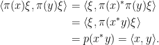
Proof: Any extension ${\tilde\pi}$ satisfies

$\displaystyle \tilde\pi(1)\pi(a)\xi=\tilde\pi(1)\tilde\pi(a)\xi=\pi(a)\xi$

so, as ${\xi}$ is cyclic for ${\mathcal A}$ , ${\tilde\pi(1)=1}$ . Hence, ${\tilde\pi(\lambda+a)=\lambda+\pi(a)}$ is the unique extension of ${\pi}$ to a *-homomorphism from ${{\mathbb C}\oplus\mathcal A}$ . As ${\lVert\xi\rVert=1}$ by corollary 6,

$\displaystyle \setlength\arraycolsep{2pt} \begin{array}{rl} \displaystyle \langle\xi,\tilde\pi(\lambda+a)\xi\rangle&\displaystyle=\lambda\langle\xi,\xi\rangle+\langle\xi,\pi(a)\xi\rangle\smallskip\\ &\displaystyle=\lambda+p(a)=p(\lambda+a) \end{array}$

as required. ⬜

Next, the GNS representation is functorial. A homomorphism between *-probability spaces is a state preserving *-homomorphism of their *-algebras, and these canonically induce isometries of their GNS Hilbert spaces.

Lemma 9 Let ${\varphi}$ be a homomorphism of bounded *-probability spaces ${(\mathcal A,p)}$ and ${(\mathcal A^\prime,p^\prime)}$ , which have GNS representations ${(\mathcal H,\pi,\xi)}$ and ${(\mathcal H^\prime,\pi^\prime,\xi^\prime)}$ respectively. Then, there exists a unique isometric linear map ${L\colon\mathcal H\rightarrow\mathcal H^\prime}$ satisfying

$\displaystyle \setlength\arraycolsep{2pt} \begin{array}{rl} &\displaystyle L\pi(a)=\pi^\prime(\varphi(a))L,\smallskip\\ &\displaystyle L\xi=\xi^\prime, \end{array}$ (4)

for all ${a\in\mathcal A}$ .

Proof: Let ${V=\{\pi(a)\xi\colon a\in\mathcal A\}}$ which, by definition, is a dense subspace of ${\mathcal H}$ . Combining equations (4),

$\displaystyle L\pi(a)\xi=\pi^\prime(\varphi(a))\xi^\prime,$

(5)

which uniquely determines ${L}$ on ${V}$ and, by continuity, this uniquely determines ${L}$ . Conversely, we can use (5) to construct ${L}$ on ${V}$ . We need to show that this is an isometry and, to be well-defined, that the right-hand-side of (5) is zero whenever ${\pi(a)\xi=0}$ . Using

$\displaystyle \setlength\arraycolsep{2pt} \begin{array}{rl} \displaystyle \lVert\pi^\prime(\varphi(a))\xi^\prime\rVert^2 &\displaystyle=\langle\xi^\prime,\pi^\prime(\varphi(a))^*\pi^\prime(\varphi(a))\xi^\prime\rangle\smallskip\\ &\displaystyle=\langle\xi^\prime,\pi^\prime(\varphi(a^*a))\xi^\prime\rangle\smallskip\\ &\displaystyle=p^\prime(\varphi(a^*a)) =p(a^*a)\smallskip\\ &\displaystyle=\langle\xi,\pi(a^*a)\xi\rangle\smallskip\\ &\displaystyle=\lVert\pi(a)\xi\rVert^2, \end{array}$

we see that ${L}$ is well-defined and an isometry. Hence, by continuous linear extension it uniquely extends to an isometry ${L\colon\mathcal H\rightarrow\mathcal H^\prime}$ . Next, we show that (4) is satisfied. Using

$\displaystyle \setlength\arraycolsep{2pt} \begin{array}{rl} \displaystyle L\pi(a)\pi(b)\xi&\displaystyle=L\pi(ab)\xi=\pi^\prime(\varphi(ab))\xi^\prime\smallskip\\ &\displaystyle=\pi^\prime(\varphi(a))\pi^\prime(\varphi(b))\xi^\prime\smallskip\\ &\displaystyle=\pi^\prime(\varphi(a))L\pi(b)\xi, \end{array}$

we see that the first identity of (4) holds on ${V}$ and, by continuity, holds on all of ${\mathcal H}$ . Finally, by extending the constructions above to ${{\mathbb C}\oplus\mathcal A}$ and ${{\mathbb C}\oplus\mathcal A^\prime}$ , we can wlog assume that ${\mathcal A}$ and ${\mathcal A^\prime}$ are unitial. Then,

$\displaystyle L\xi=L\pi(1)\xi=\pi^\prime(\varphi(1))\xi^\prime=\xi^\prime$

as required. ⬜

Finally, we put together the previous steps to complete the proof of theorem 1.

Proof of Theorem 1: The existence of the GNS representation was proven in lemma 7, so only uniqueness remains. Suppose that ${(\mathcal H,\pi,\xi)}$ and ${(\mathcal H^\prime,\pi^\prime,\xi^\prime)}$ are two GNS representations. Applying lemma 9 to the identity map ${\varphi}$ on ${\mathcal A}$ gives a unique isometry ${L\colon\mathcal H\rightarrow\mathcal H^\prime}$ satisfying ${L\pi(a)=\pi^\prime(a)L}$ and ${L\xi=\xi^\prime}$ . Similarly, there is a unique isometry ${L^\prime\colon\mathcal H^\prime\rightarrow\mathcal H}$ satisfying ${L^\prime\pi^\prime(a)=\pi(a)L^\prime}$ and ${L^\prime\xi^\prime=\xi}$ . Then, ${\tilde L=L^\prime L}$ satisfies ${\tilde L\pi(a)\xi=\pi(a)\xi}$ and, hence, is the identity map. Similarly, ${LL^\prime}$ is the identity, so ${L}$ is invertible. ⬜

	Harry on Filtrations and Adapted P…
	Anonymous on Analytic Sets
	Daniel on Analytic Sets
	Sid on Martingale Convergence
	northwiz on Preservation of the Local Mart…
	George Lowther on Martingale Convergence
	Sid on Martingale Convergence
	George Lowther on The Burkholder-Davis-Gundy Ine…
	George Lowther on Preservation of the Local Mart…
	northwiz on Preservation of the Local Mart…

The GNS Representation

Published by George Lowther

Leave a Reply Cancel reply

Like this:

Related

Published by George Lowther

Leave a Reply Cancel reply