Optional Sampling

Doob’s optional sampling theorem states that the properties of martingales, submartingales and supermartingales generalize to stopping times. For simple stopping times, which take only finitely many values in ${{\mathbb R}_+}$ , the argument is a relatively basic application of elementary integrals. For simple stopping times ${\sigma\le\tau}$ , the stochastic interval ${(\sigma,\tau]}$ and its indicator function ${1_{(\sigma,\tau]}}$ are elementary predictable. For any submartingale ${X}$ , the properties of elementary integrals give the inequality

$\displaystyle {\mathbb E}\left[X_\tau-X_\sigma\right]={\mathbb E}\left[\int_0^\infty 1_{(\sigma,\tau]}\,dX\right]\ge 0.$

(1)

For a set ${A\in \mathcal{F}_\sigma}$ the following

$\displaystyle \sigma^\prime(\omega)=\begin{cases} \sigma(\omega),&\textrm{if }\omega\in A,\\ \tau(\omega),&\textrm{otherwise}, \end{cases}$

is easily seen to be a stopping time. Replacing ${\sigma}$ by ${\sigma^\prime}$ extends inequality (1) to the following,

$\displaystyle {\mathbb E}\left[1_A(X_\tau-X_\sigma)\right]={\mathbb E}\left[X_\tau-X_{\sigma^\prime}\right]\ge 0.$

(2)

As this inequality holds for all sets ${A\in\mathcal{F}_\sigma}$ it implies the extension of the submartingale property ${X_\sigma\le{\mathbb E}[X_\tau\vert\mathcal{F}_\sigma]}$ to the random times. This argument applies to all simple stopping times, and is sufficient to prove the optional sampling result for discrete time submartingales. In continuous time, the additional hypothesis that the process is right-continuous is required. Then, the result follows by taking limits of simple stopping times.

Theorem 1 Let ${\sigma\le\tau}$ be bounded stopping times. For any cadlag martingale, submartingale or supermartingale ${X}$ , the random variables ${X_\sigma, X_\tau}$ are integrable and the following are satisfied.

If ${X}$ is a martingale then, ${X_\sigma={\mathbb E}\left[X_{\tau}\vert\mathcal{F}_\sigma\right].}$

If ${X}$ is a submartingale then, ${X_\sigma\le{\mathbb E}\left[X_{\tau}\vert\mathcal{F}_\sigma\right].}$

If ${X}$ is a supermartingale then, ${X_\sigma\ge{\mathbb E}\left[X_{\tau}\vert\mathcal{F}_\sigma\right].}$

Continue reading “Optional Sampling” →

Cadlag Modifications

As was mentioned in the initial post of these stochastic calculus notes, it is important to choose good versions of stochastic processes. In some cases, such as with Brownian motion, it is possible to explicitly construct the process to be continuous. However, in many more cases, it is necessary to appeal to more general results to assure the existence of such modifications.

The theorem below guarantees that many of the processes studied in stochastic calculus have a right-continuous version and, furthermore, these versions necessarily have left limits everywhere. Such processes are known as càdlàg from the French for “continu à droite, limites à gauche” (I often drop the accents, as seems common). Alternative terms used to refer to a cadlag process are rcll (right-continuous with left limits), R-process and right process. For a cadlag process ${X}$ , the left limit at any time ${t>0}$ is denoted by ${X_{t-}}$ (and ${X_{0-}\equiv X_0}$ ). The jump at time ${t}$ is denoted by ${\Delta X_t=X_t-X_{t-}}$ .

We work with respect to a complete filtered probability space ${(\Omega,\mathcal{F},\{\mathcal{F}_t\}_{t\ge 0},{\mathbb P})}$ .

Theorem 1 below provides us with cadlag versions under the condition that elementary integrals of the processes cannot, in a sense, get too large. Recall that elementary predictable processes are of the form

$\displaystyle \xi=Z_01_{\{t=0\}}+\sum_{k=1}^nZ_k1_{\{s_k<t\le t_k\}}$

for times ${s_k<t_k}$ , ${\mathcal{F}_0}$ -measurable random variable ${Z_0}$ and ${\mathcal{F}_{s_k}}$ -measurable random variables ${Z_k}$ . Its integral with respect to a stochastic process ${X}$ is

$\displaystyle \int_0^t \xi\,dX=\sum_{k=1}^nZ_k(X_{t_k\wedge t}-X_{s_{k}\wedge t}).$

An elementary predictable set is a subset of ${{\mathbb R}_+\times\Omega}$ which is a finite union of sets of the form ${\{0\}\times F}$ for ${F\in\mathcal{F}_0}$ and ${(s,t]\times F}$ for nonnegative reals ${s<t}$ and ${F\in\mathcal{F}_s}$ . Then, a process is an indicator function ${1_A}$ of some elementary predictable set ${A}$ if and only if it is elementary predictable and takes values in ${\{0,1\}}$ .

The following theorem guarantees the existence of cadlag versions for many types of processes. The first statement applies in particular to martingales, submartingales and supermartingales, whereas the second statement is important for the study of general semimartingales.

Theorem 1 Let X be an adapted stochastic process which is right-continuous in probability and such that either of the following conditions holds. Then, it has a cadlag version.

X is integrable and, for every ${t\in{\mathbb R}_+}$ ,
$\displaystyle \left\{{\mathbb E}\left[\int_0^t1_A\,dX\right]\colon A\textrm{ is elementary}\right\}$

is bounded.

For every ${t\in{\mathbb R}_+}$ the set
$\displaystyle \left\{\int_0^t1_A\,dX\colon A\textrm{ is elementary}\right\}$

is bounded in probability.

Continue reading “Cadlag Modifications” →

Upcrossings, Downcrossings, and Martingale Convergence

The number of times that a process passes upwards or downwards through an interval is refered to as the number of upcrossings and respectively the number of downcrossings of the process.

Consider a process ${X_t}$ whose time index ${t}$ runs through an index set ${\mathbb{T}\subseteq{\mathbb R}}$ . For real numbers ${a<b}$ , the number of upcrossings of ${X}$ across the interval ${[a,b]}$ is the supremum of the nonnegative integers ${n}$ such that there exists times ${s_k,t_k\in\mathbb{T}}$ satisfying

$\displaystyle s_1<t_1<s_2<t_2<\cdots<s_n<t_n$

(1)

and for which ${X_{s_k}\le a<b\le X_{t_k}}$ . The number of upcrossings is denoted by ${U[a,b]}$ , which is either a nonnegative integer or is infinite. Similarly, the number of downcrossings, denoted by ${D[a,b]}$ , is the supremum of the nonnegative integers ${n}$ such that there are times ${s_k,t_k\in\mathbb{T}}$ satisfying (1) and such that ${X_{s_k}\ge b>a\ge X_{t_k}}$ .

Note that between any two upcrossings there is a downcrossing and, similarly, between any two downcrossings there is an upcrossing. It follows that ${U[a,b]}$ and ${D[a,b]}$ can differ by at most 1, and they are either both finite or both infinite.

The significance of the upcrossings of a process to convergence results is due to the following criterion for convergence of a sequence.

Theorem 1 A sequence ${x_1,x_2,\ldots}$ converges to a limit in the extended real numbers if and only if the number of upcrossings ${U[a,b]}$ is finite for all ${a<b}$ .

Continue reading “Upcrossings, Downcrossings, and Martingale Convergence” →

Martingales and Elementary Integrals

A martingale is a stochastic process which stays the same, on average. That is, the expected future value conditional on the present is equal to the current value. Examples include the wealth of a gambler as a function of time, assuming that he is playing a fair game. The canonical example of a continuous time martingale is Brownian motion and, in discrete time, a symmetric random walk is a martingale. As always, we work with respect to a filtered probability space ${(\Omega,\mathcal{F},\{\mathcal{F}_t\}_{t\ge 0},{\mathbb P})}$ . A process ${X}$ is said to be integrable if the random variables ${X_t}$ are integrable, so that ${{\mathbb E}[\vert X_t\vert]<\infty}$ .

Definition 1 A martingale, ${X}$ , is an integrable process satisfying

$\displaystyle X_s={\mathbb E}[X_t\mid\mathcal{F}_s]$

for all ${s<t\in{\mathbb R}_+}$ .

Continue reading “Martingales and Elementary Integrals” →

Predictable Stopping Times

The concept of a stopping times was introduced a couple of posts back. Roughly speaking, these are times for which it is possible to observe when they occur. Often, however, it is useful to distinguish between different types of stopping times. A random time for which it is possible to predict when it is about to occur is called a predictable stopping time. As always, we work with respect to a filtered probability space ${(\Omega,\mathcal{F},\{\mathcal{F}_t\}_{t\ge 0},{\mathbb P})}$ .

Definition 1 A map ${\tau\colon\Omega\rightarrow\bar{\mathbb R}_+}$ is a predictable stopping time if there exists a sequence of stopping times ${\tau_n\uparrow\tau}$ satisfying ${\tau_n<\tau}$ whenever ${\tau\not=0}$ .

Predictable stopping times are alternatively referred to as previsible. The sequence of times ${\tau_n}$ in this definition are said to announce ${\tau}$ . Note that, in this definition, the random time was not explicitly required to be a stopping time. However, this is automatically the case, as the following equation shows.

$\displaystyle \left\{\tau\le t\right\}=\bigcap_n\left\{\tau_n\le t\right\}\in\mathcal{F}_t.$

One way in which predictable stopping times occur is as hitting times of a continuous adapted process. It is easy to predict when such a process is about to hit any level, because it must continuously approach that value.

Theorem 2 Let ${X}$ be a continuous adapted process and ${K}$ be a real number. Then

$\displaystyle \tau=\inf\left\{t\in{\mathbb R}_+\colon X_t\ge K\right\}$

is a predictable stopping time.

Proof: Let ${\tau_n}$ be the first time at which 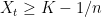${X_t\ge K-1/n}$ which, by the debut theorem, is a stopping time. This gives an increasing sequence bounded above by ${\tau}$ . Also, ${X_{\tau_n}\ge K-1/n}$ whenever ${\tau_n<\infty}$ and, by left-continuity, setting ${\sigma=\lim_n\tau_n}$ gives ${X_\sigma\ge K}$ whenever ${\sigma<\infty}$ . So, ${\sigma\ge\tau}$ , showing that the sequence ${\tau_n}$ increases to ${\tau}$ . If ${0<\tau_n\le\tau<\infty}$ then, by continuity, ${X_{\tau_n}=K-1/n\not=K=X_{\tau}}$ . So, ${\tau_n<\tau}$ whenever ${0<\tau<\infty}$ and the sequence ${n\wedge\tau_n}$ announces ${\tau}$ . ⬜

In fact, predictable stopping times are always hitting times of continuous processes, as stated by the following result. Furthermore, by the second condition below, it is enough to prove the much weaker condition that a random time can be announced `in probability’ to conclude that it is a predictable stopping time.

Lemma 3 Suppose that the filtration is complete and ${\tau\colon\Omega\rightarrow\bar{\mathbb R}_+}$ is a random time. The following are equivalent.

${\tau}$ is a predictable stopping time.

For any ${\epsilon,\delta,K>0}$ there is a stopping time ${\sigma}$ satisfying

$\displaystyle {\mathbb P}\left(K\wedge\tau-\epsilon<\sigma<\tau{\rm\ or\ }\sigma=\tau=0\right)>1-\delta.$ (1)

${\tau=\inf\{t\ge 0\colon X_t=0\}}$ for some continuous adapted process ${X}$ .

Continue reading “Predictable Stopping Times” →

Sigma Algebras at a Stopping Time

The previous post introduced the notion of a stopping time ${\tau}$ . A stochastic process ${X}$ can be sampled at such random times and, if the process is jointly measurable, ${X_\tau}$ will be a measurable random variable. It is usual to study adapted processes, where ${X_t}$ is measurable with respect to the sigma-algebra ${\mathcal{F}_t}$ at that time. Then, it is natural to extend the notion of adapted processes to random times and ask the following. What is the sigma-algebra of observable events at the random time ${\tau}$ , and is ${X_\tau}$ measurable with respect to this? The idea is that if a set ${A}$ is observable at time ${\tau}$ then for any time ${t}$ , its restriction to the set ${\{\tau\le t\}}$ should be in ${\mathcal{F}_t}$ . As always, we work with respect to a filtered probability space ${(\Omega,\mathcal{F},\{\mathcal{F}_t\}_{t\ge 0},{\mathbb P})}$ . The sigma-algebra at the stopping time ${\tau}$ is then,

$\displaystyle \mathcal{F}_\tau=\left\{A\in\mathcal{F}_\infty\colon A\cap\{\tau\le t\}\in\mathcal{F}_t{\rm\ for\ all\ }t\ge 0\right\}.$

The restriction to sets in ${\mathcal{F}_\infty}$ is to take account of the possibility that the stopping time can be infinite, and it ensures that ${A=A\cap\{\tau\le\infty\}\in\mathcal{F}_\infty}$ . From this definition, a random variable ${U}$ us ${\mathcal{F}_\tau}$ -measurable if and only if ${1_{\{\tau\le t\}}U}$ is ${\mathcal{F}_t}$ -measurable for all times ${t\in{\mathbb R}_+\cup\{\infty\}}$ .

Similarly, we can ask what is the set of events observable strictly before the stopping time. For any time ${t}$ , then this sigma-algebra should include ${\mathcal{F}_t}$ restricted to the event ${\{t<\tau\}}$ . This suggests the following definition,

$\displaystyle \mathcal{F}_{\tau-}=\sigma\left(\left\{ A\cap\{t<\tau\}\colon t\ge 0,A\in\mathcal{F}_t \right\}\cup\mathcal{F}_0\right).$

The notation ${\sigma(\cdot)}$ denotes the sigma-algebra generated by a collection of sets, and in this definition the collection of elements of ${\mathcal{F}_0}$ are included in the sigma-algebra so that we are consistent with the convention ${\mathcal{F}_{0-}=\mathcal{F}_0}$ used in these notes.

With these definitions, the question of whether or not a process ${X}$ is ${\mathcal{F}_\tau}$ -measurable at a stopping time ${\tau}$ can be answered. There is one minor issue here though; stopping times can be infinite whereas stochastic processes in these notes are defined on the time index set ${{\mathbb R}_+}$ . We could just restrict to the set ${\{\tau<\infty\}}$ , but it is handy to allow the processes to take values at infinity. So, for the moment we consider a processes ${X_t}$ where the time index ${t}$ runs over ${\bar{\mathbb R}_+\equiv{\mathbb R}_+\cup\{\infty\}}$ , and say that ${X}$ is a predictable, optional or progressive process if it satisfies the respective property restricted to times in ${{\mathbb R}_+}$ and ${X_\infty}$ is ${\mathcal{F}_\infty}$ -measurable.

Lemma 1 Let ${X}$ be a stochastic process and ${\tau}$ be a stopping time.

If ${X}$ is progressively measurable then ${X_\tau}$ is ${\mathcal{F}_\tau}$ -measurable.

If ${X}$ is predictable then ${X_\tau}$ is ${\mathcal{F}_{\tau-}}$ -measurable.

Continue reading “Sigma Algebras at a Stopping Time” →

Stopping Times and the Debut Theorem

In the previous two posts of the stochastic calculus notes, I began by introducing the basic concepts of a stochastic process and filtrations. As we often observe stochastic processes at a random time, a further definition is required. A stopping time is a random time which is adapted to the underlying filtration. As discussed in the previous post, we are working with respect to a filtered probability space ${(\Omega,\mathcal{F},\{\mathcal{F}_t\}_{t\ge 0},{\mathbb P})}$ .

Definition 1 A stopping time is a map ${\tau\colon\Omega\rightarrow{\mathbb R}_+\cup\{\infty\}}$ such that ${\{\tau\le t\}\in\mathcal{F}_t}$ for each ${t\ge 0}$ .

This definition is equivalent to stating that the process ${1_{[\tau,\infty)}}$ is adapted. Equivalently, at any time ${t}$ , the event ${\{\tau\le t\}}$ that the stopping time has already occurred is observable.

One common way in which stopping times appear is as the first time at which an adapted stochastic process hits some value. The debut theorem states that this does indeed give a stopping time.

Theorem 2 (Debut theorem) Let ${X}$ be an adapted right-continuous stochastic process defined on a complete filtered probability space. If ${K}$ is any real number then ${\tau\colon\Omega\rightarrow{\mathbb R}_+\cup\{\infty\}}$ defined by

$\displaystyle \tau(\omega)=\inf\left\{t\in{\mathbb R}_+\colon X_t(\omega)\ge K\right\}$ (1)

is a stopping time.

Continue reading “Stopping Times and the Debut Theorem” →

Filtrations and Adapted Processes

In the previous post I started by introducing the concept of a stochastic process, and their modifications. It is necessary to introduce a further concept, to represent the information available at each time. A filtration ${\{\mathcal{F}_t\}_{t\ge 0}}$ on a probability space ${(\Omega,\mathcal{F},{\mathbb P})}$ is a collection of sub-sigma-algebras of ${\mathcal{F}}$ satisfying ${\mathcal{F}_s\subseteq\mathcal{F}_t}$ whenever ${s\le t}$ . The idea is that ${\mathcal{F}_t}$ represents the set of events observable by time ${t}$ . The probability space taken together with the filtration ${(\Omega,\mathcal{F},\{\mathcal{F}_t\}_{t\ge 0},{\mathbb P})}$ is called a filtered probability space.

Given a filtration, its right and left limits at any time and the limit at infinity are as follows

$\displaystyle \mathcal{F}_{t+}=\bigcap_{s>t}\mathcal{F}_s,\ \mathcal{F}_{t-}=\sigma\Big(\bigcup_{s<t}\mathcal{F}_s\Big),\ \mathcal{F}_{\infty}=\sigma\Big(\bigcup_{t\in{\mathbb R}_+}\mathcal{F}_t\Big).$

Here, ${\sigma(\cdot)}$ denotes the sigma-algebra generated by a collection of sets. The left limit as defined here only really makes sense at positive times. Throughout these notes, I define the left limit at time zero as ${\mathcal{F}_{0-}\equiv\mathcal{F}_0}$ . The filtration is said to be right-continuous if ${\mathcal{F}_t=\mathcal{F}_{t+}}$ . Continue reading “Filtrations and Adapted Processes” →

Stochastic Processes, Indistinguishability and Modifications

I start these notes on stochastic calculus with the definition of a continuous time stochastic process. Very simply, a stochastic process is a collection of random variables ${\{X_t\}_{t\ge 0}}$ defined on a probability space ${(\Omega,\mathcal{F},{\mathbb P})}$ . That is, for each time ${t\ge 0}$ , ${\omega\mapsto X_t(\omega)}$ is a measurable function from ${\Omega}$ to the real numbers.

Stochastic processes may also take values in any measurable space ${(E,\mathcal{E})}$ but, in these notes, I concentrate on real valued processes. I am also restricting to the case where the time index ${t}$ runs through the non-negative real numbers ${{\mathbb R}_+}$ , although everything can easily be generalized to other subsets of the reals.

A stochastic process ${X\equiv\{X_t\}_{t\ge 0}}$ can be viewed in either of the following three ways.

As a collection of random variables, one for each time ${t\ge 0}$ .
As a path
$\displaystyle \setlength\arraycolsep{2pt} \begin{array}{rl} &\displaystyle {\mathbb R}_+\rightarrow{\mathbb R},\smallskip\\ &\displaystyle t\mapsto X_t(\omega), \end{array}$

one for each ${\omega\in\Omega}$ . These are referred to as the sample paths of the process.
As a function from the product space
$\displaystyle \setlength\arraycolsep{2pt} \begin{array}{rl} &\displaystyle {\mathbb R}_+\times\Omega\rightarrow{\mathbb R},\smallskip\\ &\displaystyle (t,\omega)\mapsto X_t(\omega). \end{array}$

Continue reading “Stochastic Processes, Indistinguishability and Modifications” →

Stochastic Calculus Notes

I have decided to use my blog to post some notes that I initially made on stochastic calculus when learning the subject myself. I wrote these after reading through some books which took an unnecessarily long and difficult route to get to the interesting stuff which I was interested in. Complicated and rather obscure subjects such as optional and predictable projection and a lot of theory of continuous-time martingales were dealt with at length before getting round to the general theory of stochastic integration. Consequently, I decided to go through the theory myself in a more direct way, while still working out rigorous proofs of all the more useful theorems which I was interested in learning. The result was three small notepads containing the following.

Basic definitions regarding continuous-time filtrations, adapted processes, predictable processes, stopping times, martingales, etc.
Some useful elementary results such as the debut theorem for right continuous processes and the existence of cadlag versions of martingales
Definition of stochastic integration and elementary properties.
Definition and elementary properties of quadratic variations.
Ito’s formula, including the generalized Ito formula for non-continuous processes.
Stochastic integration with respect to martingales.
The Doob-Meyer decomposition.
Quasimartingale decompositions.
Decompositions of semimartingales.
Decompositions and integration with respect to special semimartingales.

This covers a lot of the general underlying theory required. Of course, being able to apply this to practical applications requires further knowledge of stuff like stochastic differential equations. Time permitting, I’ll start to post these notes here.As I have learned much more since originally making these notes, I will attempt to simplify or improve on the originals where possible.

The prerequisite knowledge required to properly understand these notes is measure theoretic probability theory (e.g., properties of the Lebesgue integral such as dominated convergence, Fubini’s theorem, $L^p$ spaces, convergence in probability, etc.).

	Anonymous on Spitzer’s Formula
	Anonymous on Spitzer’s Formula
	Anonymous on Brownian Bridges
	Anonymous on Spitzer’s Formula
	Anonymous on Spitzer’s Formula
	Anonymous on Spitzer’s Formula
	Anonymous on Spitzer’s Formula
	Anonymous on Spitzer’s Formula
	Anonymous on Spitzer’s Formula
	Anonymous on Spitzer’s Formula