In the previous post I started by introducing the concept of a stochastic process, and their modifications. It is necessary to introduce a further concept, to represent the information available at each time. A filtration 


Given a filtration, its right and left limits at any time and the limit at infinity are as follows
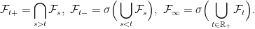
Here, 


A probability space 


Often, in stochastic process theory, filtered probability spaces are assumed to satisfy the usual conditions, meaning that it is complete and the filtration is right-continuous. Note that any filtered probability space can be completed simply by completing the underlying probability space and then adding all zero probability sets to each 
Throughout these notes I assume a complete filtered probability space, although many of the results can be extended to the non-complete case without much difficulty. However, for the sake of a bit more generality, I don’t assume that filtrations are right-continuous.
One reason for using filtrations is to define adapted processes. A stochastic process process 


As mentioned in the previous post, it is often necessary to impose measurability constraints on a process 
Definition 1
- The predictable sigma-algebra on
, denoted by
, is generated by the left-continuous and adapted processes. A stochastic process is said to be predictable if it is
- The optional sigma-algebra on
, is generated by the right-continuous and adapted processes. A stochastic process is said to be optional if it is
- A process
is
-measurable.
![\displaystyle \setlength\arraycolsep{2pt} \begin{array}{rl} &\displaystyle [0,t]\times\Omega\rightarrow{\mathbb R},\smallskip\\ &\displaystyle (s,\omega)\mapsto X_s(\omega) \end{array}](https://s0.wp.com/latex.php?latex=%5Cdisplaystyle++%5Csetlength%5Carraycolsep%7B2pt%7D+%5Cbegin%7Barray%7D%7Brl%7D+%26%5Cdisplaystyle+%5B0%2Ct%5D%5Ctimes%5COmega%5Crightarrow%7B%5Cmathbb+R%7D%2C%5Csmallskip%5C%5C+%26%5Cdisplaystyle+%28s%2C%5Comega%29%5Cmapsto+X_s%28%5Comega%29+%5Cend%7Barray%7D+&bg=ffffff&fg=000000&s=0&c=20201002)
The most important of these definitions, at least in these notes, is that of predictable processes. While adapted right-continuous processes will be used extensively, there is not much need to generalize to optional processes. Similarly, progressive measurability isn’t used a lot except in the context of adapted right-continuous (and therefore optional) processes. On the other hand, predictable processes are extensively used as integrands for stochastic integrals and in the Doob-Meyer decomposition, and are often not restricted to the adapted and left-continuous case.
Given any set of real-valued functions on a set, which is closed under multiplication, the set of functions measurable with respect to the generated sigma-algebra can be identitified as follows. They form the smallest set of real-valued functions containing the generating set and which is closed under taking linear combinations and increasing limits. So, for example, the predictable processes form the smallest set containing the adapted left-continuous processes which is closed under linear combinations and such that the limit of an increasing sequence of predictable processes is predictable.
Another way of defining predictable processes is in terms of continuous adapted processes.
Lemma 2 The predictable sigma-algebra is generated by the continuous and adapted processes.
Proof: Clearly every continuous adapted process is left-continuous and, therefore, is predictable. Conversely, if
Continuity of 


A further method of defining the predictable sigma-algebra is in terms of simple sets generating it. The following is sometimes used.
Lemma 3 The predictable sigma-algebra is generated by the sets of the form
(1)
![\displaystyle \left\{(s,t]\times A\colon t>s\ge 0, A\in\mathcal{F}_s\right\}\cup\left\{\{0\}\times A\colon A\in\mathcal{F}_0\right\}.](https://s0.wp.com/latex.php?latex=%5Cdisplaystyle++%5Cleft%5C%7B%28s%2Ct%5D%5Ctimes+A%5Ccolon+t%3Es%5Cge+0%2C+A%5Cin%5Cmathcal%7BF%7D_s%5Cright%5C%7D%5Ccup%5Cleft%5C%7B%5C%7B0%5C%7D%5Ctimes+A%5Ccolon+A%5Cin%5Cmathcal%7BF%7D_0%5Cright%5C%7D.+&bg=ffffff&fg=000000&s=0&c=20201002)
Proof: If 


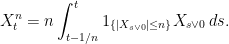
Conversely, let X be left-continuous and adapted. Then it is the limit of the piecewise constant functions

as n goes to infinity. Each of the summands on the right hand side is easily seen to be measurable with respect to the sigma-algebra generated by the collection (1). So, 
In these notes, I refer to the collection of finite unions of sets in the collection (1) as the elementary or elementary predictable sets. Writing these as 

Finally, the different forms of measurability can be listed in order of generality, starting with the predictable processes, up to the much larger class of jointly measurable adapted processes.
Lemma 4 Each of the following properties of a stochastic process implies the next
- predictable.
- optional.
- progressive.
- adapted and jointly measurable.
Proof: As the predictable sigma-algebra is generated by the continuous adapted processes, which are also optional by definition, it follows that all predictable processes are optional.
Now, if 


Finally, consider a progressively measurable process 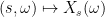
![{[0,t]\times\Omega}](https://s0.wp.com/latex.php?latex=%7B%5B0%2Ct%5D%5Ctimes%5COmega%7D&bg=ffffff&fg=000000&s=0&c=20201002)


I have been trying to find clarification on a question relating to filtrations and measurability for awhile, but can’t find discussions of it. I figure someone knowledgeable about stochastic processes would know this. If you have a random variable X that is measurable with respect to a sigma algebra generated by random variable Y, then there exists a function g such that X=g(Y). But what if the sigma algebra is generated by an uncountable number of random variables, such as where F is the natural filtration of stochastic process Y. What can be said in this case for r.v. X measurable with respect to F_t? Is there any functional representation?
Thanks for any help.
Yes there is! Assuming that X is a real-valued random variable, then it can be expressed as a function of Y.
If Y:Ω → E is a measurable map from the underlying probability space to a measurable space (E,ℰ) then any σ(Y)-measurable map X:Ω → ℝ can be written as X = g(Y) for a measurable g:E → ℝ. This is an application of the functional monotone class theorem. (i) Show that every X = 1A for A ∈ σ(Y) is of the form g(Y). (ii) Show that the set of random variables of the form g(Y) is closed under linear combinations and taking increasing limits. (iii) appeal to the monotone class theorem.
If Yt is a (real-valued) process, it can be considered as a map to the space ℝℝ+ of real valued functions.
Hi,
According to Lemma 2, will it be true to say that all brownian motions and martingales that are continuous are predictable processes?
Yes, that’s correct. Assuming you are using an appropriate filtration, so that your processes are adapted, then they are predictable.
Thanks for your reply George.
One more thing that’s bothering me, in the context of finding an equivalent martingale measure. Correct if I am wrong below:
For discounted asset price process, Dt (assuming a constant discount rate), there are two reasons why the discounted asset price process could be predictable:
a) Dt will be a martingale under say Q-probability measure, and is hence predictable (under this probability measure only?).
b) If we assume say Geometric Brownian Motion Model for the asset price, the random component of the asset price will only be the Brownian Motion, which is predictable. Hence St (and Dt) is a predictable process.
I have read somewhere that Dt is predictable, which is not very intuitive since asset prices from the market cannot be predictable. Hence my two reasoning above: Predictable only under certain probability measure OR predictable for asset prices which we have assumed a certain model.
Hope you can understand where I am coming from and really appreciate if you could shed some light on this.
Su,
The reason why processes such as Brownian motion are predictable is just because they are continuous and adapted. It does not have anything to do with the martingale property. In fact, it does not have much to do with the measure either. The property of being predictable is not affected by an equivalent measure change.
I think maybe you are a bit confused about the meaning of being predictable in the precise mathematical sense defined above, which is rather different from the (rather ill-defined) everyday notion of something being predictable. Here, predictability only means that you can (roughly speaking) predict the future value in an infinitesimal sense. Just because a Brownian motion is predictable does not mean that you can tell what value it will take at some future point in time. What you can say is that you can tell when the process is going to reach some value a just prior to it happening. This is simply because of continuity. If at some time then, by continuity,
  will be arbitrarily small for times s just before t.
So, you can model asset prices by predictable processes. It simply means that they are continuous. Under Black-Scholes, the process is predictable in this sense. That is because it ignores the possibility that the price can suddenly jump.
And, apologies for the late response. Hope that helps clear things up a bit.
Hi George,
Appreciate the explanation. Definitely cleared things up!
Nice proof of Lemma 2, although it took me a while to see why it does not get through when X is right continuous :). Adapt.
BTW, would that mean if the filtration is right continuous, then optional sigma field = predictable sigma field?
Hi Yaoliang. The proof of Lemma 2 doesn’t work if X is only right-continuous because Xn would not converge to X. I’m not sure why you suggest that optional = predictable when the filtration is right-continuous though. This is not true. The filtration generated by a Poisson process is right-continuous (once you complete it), but Poisson processes are not predictable. However, it is often the case that optional = pedictable. For example, this happens if the filtration is generated by a Brownian motion — see my latest post Predictable Stopping Times.
Thanks, George. Here is what I thought about right continuous processes: change the integral interval of X^n from [t-1/n,t] to [t, t+1/n]. Would this be enough to argue that X^n converges to X? But of course, X is only F_+ measurable, that’s why I thought option=predictable when the filtration is right continuous (then F_+=F, hence X is adapted). I believe my claim is false, but still couldn’t see why the proof of Lemma 2 cannot go through.
Lemma 2 relies on the fact that the processes Xn are both continuous and adapted and, then, the fact that they converge to X means that X is measurable with respect to the sigma algebra generated by the continuous and adapted processes. -adapted for any given
  . This is much weaker than being measurable with respect to the continous and
  -adapted processes.
If X was only assumed to be right-continuous then, as you say, you could define Xn by integrating over the range [t,t+1/n] instead. However, Xn would not be adapted. So, you can say that X is measurable with respect to the sigma-algebra generated by the continuous processes. But, it need not be measurable with respect to the sigma-algebra generated by the processes which are simultaneously continuous and adapted. It is true though, that X is measurable with respect to the processes which are continuous and
Hi, George. You say “The filtration generated by a Poisson process is right-continuous (once you complete it)” – I know that was off-hand, but why is this the case? I’m trying to go through the mechanics of proving that statement, and it doesn’t seem to come to easily – the modulus for the right continuity of the process is stochastic.
Hi. One method to prove what you want using results from these notes, is to apply the statements that, Poisson processes are Feller and Feller processes have right-continuous filtration.
A more direct proof would be to show that![\mathbb{E}[U\vert\mathcal{F}_{t+}]=\mathbb{E}[U\vert\mathcal{F}_{t}]](https://s0.wp.com/latex.php?latex=%5Cmathbb%7BE%7D%5BU%5Cvert%5Cmathcal%7BF%7D_%7Bt%2B%7D%5D%3D%5Cmathbb%7BE%7D%5BU%5Cvert%5Cmathcal%7BF%7D_%7Bt%7D%5D&bg=ffffff&fg=000000&s=0&c=20201002) for bounded rvs U. For U a function of
for bounded rvs U. For U a function of  , with
  it follows from the independent increments property, and it is immediate for U
  measurable. It can be extended to general U using the monotone class lemma.
Thanks for the references and response, George. It seems like both approaches (Feller and the “direct proof”) only show![\mathbb{E}[U|\mathcal{F}_t]=\mathbb{E}[U|\mathcal{F}_{t+}]](https://s0.wp.com/latex.php?latex=%5Cmathbb%7BE%7D%5BU%7C%5Cmathcal%7BF%7D_t%5D%3D%5Cmathbb%7BE%7D%5BU%7C%5Cmathcal%7BF%7D_%7Bt%2B%7D%5D&bg=ffffff&fg=000000&s=0&c=20201002) almost surely, which is fine if the
almost surely, which is fine if the  -algebras are known to be augmented already. However, in the natural filtration
  for a Poisson process is trivial, so it would seem that any approach showing conditional expectations are equivalent would suffer from the augmentation assumption. Is this assumption tight? I’d imagine so.
Something still seems off for the direct proof sketch, even with augmentation, though – why couldn’t we apply it to the augmented natural filtration for the Wiener process, which isn’t RC?
By the ‘augmented’ natural filtration, you just mean with the zero probability events added, right? In that case, the argument shows that the augmented natural filtration is right-continuous. The argument does indeed apply to the Wiener process, whose augmented natural filtration is right-continuous.
I was not making any claim about the non-augmented natural filtration although, now I think about it, it will still be right-continuous for the Poissoj process (but, not for the Wiener process).
Hi George,
Thanks for this great post, it certainly clears things up. Nevertheless I have some trouble understanding the proof of lemma 4. I don’t completely understand how optional impies progressive. You proved that the generators of the optional sigma algebra, are progressively measurable. But I don’t see how this implies that for any optional process this also holds. Do you assume if the generators of a sigma algebra are B([o,t]) x Ft measurable on the subset [0,t] x omega then the same holds for the functions measurable with respect to this sigma algebra? I hope you understand my problem, and I would really appreciate it if you would explain this to me.
All the best,
GuidovM
GuidovM,
Yes I did assume that if the generators of a sigma algebra are B([0,t]) × Ft measurable on the subset [0,t] × Ω then the same holds for the functions measurable with respect to this sigma algebra.
Maybe I did not explain this bit well. You can show that the sets A ⊆ R+×Ω which are B([0,t])×Ft measurable on the subsets [0,t] × Ω forms a sigma-algebra (just check that it is closed under countable unions and taking complements). This is the progressive sigma-algebra. Furthermore, the definition of progressive processes given in Definition 1 is equivalent to saying that the process is measurable with respect to the progressive sigma-algebra. So, the statement “optional ⇒ progressive” is the same as saying that optional sigma-algebra ⊆ progressive sigma-algebra. To prove this you only need to look at processes generating the optional sigma-algebra.
I should add a statement to Definition 1 defining the progressive sigma-algebra and stating that progressive ⇔ measurable with respect to the progressive sigma-algebra. I’ll do this at some point – thanks for mentioning it.
Hope that clears things up.
Hi George,
Regarding the construction of the mentioned progressive sigma-algebra, I can easily verify that it is closed under countable unions. But it is not that trivial to me that it is also closed under taking complements. Could you please explain this more explicitly to a beginner? Thanks a lot!
Hi George,
First of all thanks for your great set of notes. They are among the best I have come across so far.
Quick question:
Is it true that if a function f is F1xF2 measurable and that its section f_y(x) is F1* measurable for all y in Omega2, then f is F1xF2* measurable?
Your proof of “optional => progressive” seems to rely on the latter fact.
Thanks in advance!
– Tigran
Actually I just realized that your proof does not require what I mentioned.
Never mind!
Hi.
No, I don’t rely on that fact. Actually, that’s not true. Consider for example F1, F2 to be the Borel sigma-algebra on the reals. Let f be the indicator function of a non-measurable subset of the diagonal in R2. Then, fy(x) will be measurable for each y, but f itself is not measurable (I’m not sure what you mean by F1* and F1xF2*. Maybe the completion? That depends on having a measure though).
Thanks for the reply. I realized after my initial comment that the proof doesn’t rely on this statement.
I also just realized how unclear my initial statement actually was (and how inconsistent the notation was as well).
What I meant to say is that suppose f(x,y) is measurable w.r.t. some joint sigma-algebra (F1xF2) and that its section in y (f_y(x)) is measurable w.r.t. a sigma-algebra smaller than F1 (this smaller sigma-algebra is denoted F1*) for each y.
Note: F1* does not depend on y.
The question is: Is f(x,y) measurable w.r.t. F1*xF2?
I have a feeling the answer in no.
The answer is indeed no. Consider any probability space (Ω,F1,P) on which we have defined a uniformly distributed random variable T: Ω → [0,1]. Let F1* consist of the sets in F1 with probability 0 or 1. Let F2 be the Borel sigma-algebra on [0,1].
Now, look at the stochastic process Ω×[0,1] → R given by (ω,t) ↦ Xt(ω) = 1{T(ω)=t}. This is F1×F2 measurable but not F1*×F2 measurable. However, Xt is almost surely zero at each time t, so is F1* measurable.
Thanks again for your answer George. It’s a nice counter-example.
The only bit that I have yet to understand completely is: why is I_{T(omega}=t} not F1*xF2-measurable.
It’s probably a trivial detail that I am missing and your input would be great to help me understand this.
P.S.: Once again my hat is off to the clarity of your notes. They are extremely helpful in getting a better intuition of the technicalities in stochastic analysis.
It is true that this process is not F1*xF2 measurable. However, it is not a trivial detail. Far from it. You can prove it by the measurable projection theorem. If it was measurable then this theorem would tell you that the set of ω ∈ Ω such that there exists a t ≤ 1/2 with Xt(ω) = 1 is measurable with respect to the completion of F1*, so has measure 0 or 1. However, this set is just {T ≤ 1/2}, which has probability 1/2. So X is not F1*xF2 measurable.
…actually the measurable projection theorem is very similar to the generalised form of the Debut theorem which says that the first time that a jointly measurable process hits a measurable set is itself measurable wrt the completion of the probability space (and is a stopping time if the process is progressive and the filtration is right continuous). In this case, the first time X hits 1 is T, which is not F1* measurable. So X is not F1*xF2 measurable.
Dear George, thanks for very nice notes – the explanation is highly helpful. I didn’t get the definition of a predictable sigma-algebra: that is generated by left-continuous and adapted processes. W.r.t. which filtration processes generating predictable sigma-algebra should be adapted?
Thanks in advance,
Ilya.
The definition of the predictable sigma-algebra does depend on what underlying filtration is used to define adapted processes. Usually, we are given one sigma-algebra (representing all observable events at time t). Then, we work exclusively with respect to this sigma-algebra, which is used in the definition of adapted processes (and predictable processes, optional processes, stopping times, etc). If we have multiple sigma-algebras and it is not clear which one is being used from the context, then it should be stated. With multiple sigma-algebras, we have multiple predictable sigma-algebras (and multiple optional sigma algebras, etc). Where this happens in these notes I say something along the lines of “the
  -predictable sigma algebra” or “predictable with respect to
  ”).
”).
Hi!
I don’t quite understand why it is important to assume the usual conditions. What exactly do we miss if don’t assume them? Do stochastic integral stop being adapted? Are we unable to make Doob-Meyer decompositions? Martingales stop having a cadlag version? When we make a Girsanov transformation, the new Brownian motion generates a filtration which does not coincide with the filtration of the original Bm?
Thanks for these great notes!
Cadlag versions and stochastic integrals would both fail to be adapted. Check: compensated Poisson process X, pick its left-continuous version Y and the filtration generated by Y (= the predictable).
George, I would like to ask a question about this very useful thread. In Lemma 2, when you define the process $X_t^n = \int_{t-1/n}^t etc… I can see that this definition works when $X_t $ is a step process or a simple process. But for general $X_t $ how do you handle them inside the integral?…. Are you saying that one should prove it using the functional monotone class theorem? In this case which version do you use as there is more than one fMonClassTheorem? Thank you in advance if you could throw a few more details in there.
Hi, I have a quite related question. Suppose X and Y are two continuous processes. For each t, Xt is adapted with respect to {Ys:s X(t,w) and (t, w) –> Y(t,w), is the joint sigma-field generated by X contained in that generated by Y? This kind of joint measurability question is interesting and difficult.
Sorry, there seems to be some system error. My question is like this: Suppose X and Y are two continuous processes. For each t, Xt is adapted with respect to {Ys:s X(t,w) and (t, w) –> Y(t,w), is the joint sigma-field generated by X contained in that generated by Y?
Sorry, still error. Suppose X and Y are two continuous processes. For each t, Xt is adapted with respect to {Ys:s< = t}.
Considering X and Y as functions (t,w) –> X(t,w) and (t, w) –> Y(t,w), is the joint sigma-field generated by X contained in that generated by Y?
Hi George Lowther
I could not understand what do you mean by the following? I would be grateful if you could explain it
“Given any set of real-valued functions on a set, which is closed under multiplication, the set of functions measurable with respect to the generated sigma-algebra can be identitified as follows. They form the smallest set of real-valued functions containing the generating set and which is closed under taking linear combinations and increasing limits. So, for example, the predictable processes form the smallest set containing the adapted left-continuous processes which is closed under linear combinations and such that the limit of an increasing sequence of predictable processes is predictable.”
In the proof of lemma 2, do you really need the functional monotone class theorem? Doesn’t continuity follow directly by choosing
I think you are correct — but why not just ?
?
Actually, I see why you used the min, but it is unnecessary. I updated the post. Thanks!
Hi George,
I have a question regarding adaptedness and filtration: is adaptedness a distributional property? is a probability space supporting a Brownian motion
  , where the filtration is the augmented brownian filtration
  and
and  . Let
. Let  be a jointly measurable process which is a martingale in its own natural filtration. I want to understand if there is condition in terms of the joint law of
  (on the canonical path space
 ![\mathcal C([0,T])\times \mathbb D([0,T])](https://s0.wp.com/latex.php?latex=%5Cmathcal+C%28%5B0%2CT%5D%29%5Ctimes+%5Cmathbb+D%28%5B0%2CT%5D%29&bg=ffffff&fg=000000&s=0&c=20201002) ) which is sufficient for
) which is sufficient for  to be
to be  -adapted.
 is a martingale w.r.t.
  , then
  is
is  -adapted. Namely I want to show that enlarge the Brownian filtration by including future information will destroy the martingale property of the brownian motion. I am wondering if this is true or not. Thanks!
More precisely, Suppose
My first guess is that if
Are you asking if any strict enlargement of the Brownian filtration (but keeping the same underlying probability space) will necessarily destroy the martingale property of the underlying Brownian motion?
If so, then yes that is true. By the martingale representation theorem, all martingale would have to retain the martingale property, in which case the result follows.
Thank you for your prompt response. As a follow-up question, I am wondering if this is still true in the discrete time case where is a random walk with jumps that are i.i.d normal random variables(say,with mean zero). I am not aware of any martingale representation in discrete time, except the binomial-tree model. Thanks again!
In the discrete time case you mention, it is possible to enlarge the filtration while keeping the martingale property. For example, add the absolute sizes of all the jumps to .
.
I agree with you that the martingale property can be preserved by enlarging the filtration. However, in this case it seems that we may lose the independent increment property(i.e., is no longer independent of
  ). Going back to my original question which involve the process
  . Is there a condition on the joint distribution of
  which will guarantee that
  is adapted to
  ? Namely, can we find two processes
  and
and  , one being adapted and one not, such that
  has the same distribution as
  ? As you pointed out this is not possible in the continuous time case.
Thank you and looking forward to your reply!
On your question about the distribution of , I would consider the statement that S is W adapted to be a statement about this distribution, so I am not sure what further to say about it.
what I am looking for is a condition on the joint distribution which can be expressed in terms of some equations. For example, that is
is  martingale is equivalent to saying
  for all f. Unfortunately, this is not sufficient to give adaptedness as you pointed out. I am just curious if one can formulate condition of this kind which is sufficient. I hope this is a question that worth thinking. thank you!
I think it should be enough to state that, for each , the distribution of
  conditional on
  Is preserved. In the case of independent increments, it is enough to say that is preserved.
Sorry that I miss the initial space in very latex code. I re-typed the comment here:
Suppose is a probability space supporting a Brownian motion
  , where the filtration is the augmented brownian filtration
  and $latex\mathcal F=F_T^W$. Let
  be a jointly measurable process which is a martingale in its own natural filtration. I want to understand if there is condition in terms of the joint law of $ latex(W,S)$ (on the canonical path space $ latex\mathcal C([0,T])\times \mathbb D([0,T])$) which is sufficient for $ latex\{S_t\}_{0 \leq t \leq T}$ to be $ latex\mathbb F$-adapted.
My first guess is that if latex$ W$ is a martingale w.r.t. the possibly larger filtration $ latex\{F_t^W \vee F_t^S \}_{0\leq t\leq T}$, then $ latex\{S_t\}_{0 \leq t \leq T}$ is $ latex\mathbb F$-adapted. Namely I want to show that enlarge the Brownian filtration by including future information will destroy the martingale property of the brownian motion. I am wondering if this is true or not. Thanks!
So sorry i miss place the space again. Please ignore the previous comment. this time i should have got it right.
Suppose is a probability space supporting a Brownian motion
  , where the filtration is the augmented brownian filtration
  and
and  . Let
. Let  be a jointly measurable process which is a martingale in its own natural filtration. I want to understand if there is condition in terms of the joint law of
  (on the canonical path space
 ![\mathcal C([0,T])\times \mathbb D([0,T])](https://s0.wp.com/latex.php?latex=%5Cmathcal+C%28%5B0%2CT%5D%29%5Ctimes+%5Cmathbb+D%28%5B0%2CT%5D%29&bg=ffffff&fg=000000&s=0&c=20201002) ) which is sufficient for
) which is sufficient for  to be
to be  -adapted.
 is a martingale w.r.t.
  , then
  is
is  -adapted. Namely I want to show that enlarge the Brownian filtration by including future information will destroy the martingale property of the brownian motion. I am wondering if this is true or not. Thanks!
My first guess is that if
Hi!
You define a predictable sigma-algebra on {{\mathbb R}_+\times\Omega}, denoted by {\mathcal{P}} to be the sigma algebra generated by the left-continuous and adapted processes. You also write that a adapted process is one which in turn depends on the sigma algebra i.e that each r.v is measuable. This seems circular to me, do you mean that we take a left contious processes and then generate it’s natural filtration? Or have I gotten something wrong?
Assume that $L$ is a process of FV that is adapted to the filtration generated by a Wiener Process $W$ defined in a probability space $(\Omega, \mathcal{F}, P)$ and consider a, say, continuous function $f:[0,T]\to\mathbb{R}$ (I have f(t)=exp(-rt) with $r>0$ in mind). Let us define the stochastic process $X_t:=\int_0^t f(t)dL_t$. Is it the case that the expectation of $X_T$ with respect to $P$ is always well defined? Many thanks!
Hello. It occurs to me that the definition of natural filtration of a rv as the smallest filtration to which it is adapted is not obviously well-defined, because there is no total order on the set of filtrations. We can define a partial order by saying that one filtration
  is less than or equal to another
  iff $\forall t\geq 0:\ \mathscr F^1_t\subseteq \mathscr F^2_t$. It is imaginable that a rv would have multiple filtrations that are minimum elements of the poset of filtrations under that order. It seems to me that the simplest way to define a natural filtration is by the formula given in the sentence that follows the definition above, ie
  . We would then wish to prove that filtration
  is smaller than any filtration to which
  is adapted, under the above-defined order. That, together with the observation that
  is adapted to that filtration, would entail that filtration
  is a unique minimum element of the subset of all filtrations to which
  is adapted.
I hope this LaTeX works. It’s the first time I’ve tried using it in a WordPress environment 🙂
Hi in my opinion what you do in the second part of your post is exactly what it means in the definition of this blog for a filtration to be minimal (and hence the natural filtration w.r.t. the process X), and being minimal has nothing to do with a total order on the set of all filtrations. So even if what you say in the second part makes sense it is redundant with the notions used here and there is no problem of definition. Best regards
It doesn’t require a total order but it does require a partial order and the existence of a minimal element of the set of adapted filtrations. Perhaps I missed it but I couldn’t see any definition of an order relation on filtrations above, which is why I suggested one (there is an implicit order relation used on sigma algebras, but not on filtrations). Having done that, it remains to be proved that the set of filtrations adapted to a process X has a minimal element under that order relation. I imagine one would do that by taking the filtration such that
  and proving that it is a minimal element under that order relation.
So far so good, you make explicit what is implicit in the post (but very clear from the context IMO). Nonetheless your precisions are exactly what the definition given here is about and I wouldn’t go as far as qualify the definition of natural filtration as not well defined (introducing pre-order is a bit overkill here). Best regards
In the proof of Lemma 2, you reason as “In fact, as is bounded by
  , it has Lipschitz constant
  .” I doubt that “boundedness” implies “Lipschitz”, the counterexample being
  on
on ![[0,1]](https://s0.wp.com/latex.php?latex=%5B0%2C1%5D&bg=ffffff&fg=000000&s=0&c=20201002) .
.
What I meant is that as f is bounded, its integral is Lipschitz.
Thanks for the helpful post! In Lemma 2, either I am missing something, or you don’t mention anywhere that the integral is adapted. It is clear though because adapted left continuous processes are progressive, and progressive processes have adapted integrals.
I stated that is adapted, but did not explicitly prove this, because I thought that it is clear. As you note, integrals of progressive processes are adapted. Alternatively, Riemann sum evaluation of the integral shows that it is adapted.
Hi George,
I have a related question, that I was not yet able to answer. If we take to be the filtration generated by a standard Brownian motion
  in
in  and we define
  , can we find an
  -adapted
  such that the filtration generated by
  is smaller than
  ?
?
Hi. Nice question! Here is a partial answer:
Let us start with a standard Brownian motion B generating filtration . Next, let S be any set which is not in
  . For example,
  . Next, let
  be the filtration generated by
  and S. By Jacod’s countable extension, B is still a semimartingale under this enlarged filtration. As its quadratic variation is
 ![[B]_t=t](https://s0.wp.com/latex.php?latex=%5BB%5D_t%3Dt&bg=ffffff&fg=000000&s=0&c=20201002) , we have
, we have  for some Brownian motion W under the enlarged filtration and continuous FV process A. Furthermore, since
  for any predictable process
  satisfying
  (a.s.), it follows that A is absolutely continuous and, hence,
  for a predictable
  .
.
So, in summary, we have a Brownian motion W and predictable adapted to filtration
  , such that
  is a Brownian motion adapted to the strictly smaller filtration
  . All that is missing is to show that
  is generated by W. However, I do not think that this is the case, and S will not be in the natural filtration of W at any time before 1.
Hi. I have an answer to your question, which is yes, we can find such a ! See this post.
Just a typo: I think that on the RHS of the main equality in the proof of lemma 3 the n’s in the superscript should be deleted.
I enjoy this site.
You are correct – I fixed it now. Thanks!
Very small typo: “are automatically jointly measurability” [George: Fixed, Thanks!]
Hi, quick question. In the proof of Lemma 2, why is bounded by
  ? If
? If  shouldn’t the bound be
  ?
?
We have . You are missing the factor of n.
Hi George, I have a question regarding your definition of optional sigma algebra. You define it as the sigma algebra generated by right-continuous adapted processes. But other references I found all define it as being generated by cadlag adapted processes. May I ask why you drop the left hand limit condition here? Does it not affect anything?
I dropped the left-hand limit condition here simply because it is easier in context (right-continuous processes generate the optional processes and left-continuous generate the predictable ones). Requiring the processes to have left-limits is a bit unintuitive and makes no practical difference. They generate the same sigma algebra in the case that the filtered probability space is complete, which I am assuming. See my post on optional processes.
If the filtered probability space is not complete, then the two definitions could differ, but only by evanescent sets.
Sorry, this is a bit late…You state that, “On the other hand, predictable processes are extensively used as integrands for stochastic integrals and in the Doob-Meyer decomposition, and are often not restricted to the adapted and left-continuous case.”. Does it mean that there are predictable processes that are not (merely) left-continuous and adapted? If so, can you please give an example?
Yes. For a rather dumb example, just take a deterministic measurable process. Eg, .
. for fixed positive h, so that its values are known a time h in advance.
For slightly more interesting examples, take any progressively measurable process X and translate it to
Hey George, this is late but I just found your site is very helpful. I’m get a bit confused from your proof in lemma 4. So you said optional algebra is generated by right continuous and adapted process, is this mean every optional process is right continuous and adapted? If not, what’s the logic behind section “optional to progressive”?
No, it means that optional processes are measurable with respect to the sigma-algebra generated by the right-continuous and adapted processes. This includes pointwise limits of sequences of such processes, limits of sequences of these limits and so on.
Thank you for the clarification! So the argument is that an optional process is a limit of right-continuous and adapted processes, which are also progressive. Then the claim follows from the fact that a limit of progressive processes is still progressive. Is that right?
almost…an optional process is not necessarily a limit of right-continuous processes. It could be a limit of limits, a limit of limits of limits, and so on. Either way, the fact that right-continuous adapted processes are progressive is enough to imply that optional processes are progressive
In the proof of a process being optional implies it being progressive, should it be![\mathcal{B}([0,T])\otimes \mathcal{F}_t](https://s0.wp.com/latex.php?latex=%5Cmathcal%7BB%7D%28%5B0%2CT%5D%29%5Cotimes+%5Cmathcal%7BF%7D_t&bg=ffffff&fg=000000&s=0&c=20201002) instead of
instead of ![\mathcal{B}([0,\infty])\otimes \mathcal{F}_t](https://s0.wp.com/latex.php?latex=%5Cmathcal%7BB%7D%28%5B0%2C%5Cinfty%5D%29%5Cotimes+%5Cmathcal%7BF%7D_t&bg=ffffff&fg=000000&s=0&c=20201002) ? Thank you in advance.
? Thank you in advance.
You mean in the proof of Lemma 4? Here, Y is defined for all times t >= 0, so is -measurable. This immediately implies that restricted to the interval [0,T] (on which it equals X) it is
 ![\mathcal B([0,T])\otimes\mathcal F_t](https://s0.wp.com/latex.php?latex=%5Cmathcal+B%28%5B0%2CT%5D%29%5Cotimes%5Cmathcal+F_t&bg=ffffff&fg=000000&s=0&c=20201002) -measurable.
-measurable.
Dear George,
Why is the measurability with respect to the product sigma algebra restricted to the interval [0,T] an immediate result? Could you please explain this more explicitly for a beginner? Thank you very much!
By the way, is there a typo regarding the subscript of the sigma algebra F_t?Should it be T instead of t?
I find your posts really insightful!!! Thanks.
In Lemma 2, you define the process $X_n^t$. You showed that this process in continuous, and converges to $X_t$. But don’t you also need to show that $X_n^t$ is adapted, i.e. $X_n^t \in \mathcal{F}_t$? It’s not clear, since the definition of $X_n^t$ involves taking an integral of $X$.
Actually I found Prop 1.13 in Karatzas and Shreve which says that every left (or right) continuous adapted process is progressively measurable. This is enough to show that the $X_n^t$ are adapted.
Apologies for the formatting, I’m not sure how to get the latex to show up properly.
X^n_t is an integral of X_s over s <= t which, by Riemann sum approximation, is a limit of linear combinations of X_s over s <= t (and linear combinations+limits preserves measurability), so is F_t-measurable.
In Lemma 2 you conclude that is measurable w.r.t.
  whenever
  . It’s not clear to me why this is true.
I can see that for any Bore set we have that
  , if
, if  means point-wise convergence on
  .
.
But you’ve used the other inclusion, i.e. , in order to conclude that
  is measurable w.r.t.
  . Why is this inclusion true?
Hi. X^n are adapted and converge to X pointwise, so X is also adapted. This is just a standard result that the pointwise limit of a set of random variables measurable wrt a sigma-algebra is itself measurable.
Note in the following post, I mention that the supremum is measurable. So
lim_n X^n = inf_{m}sup_{n > m}X^n
is also measurable.