Poisson Processes

A Poisson process is a continuous-time stochastic process which counts the arrival of randomly occurring events. Commonly cited examples which can be modeled by a Poisson process include radioactive decay of atoms and telephone calls arriving at an exchange, in which the number of events occurring in each consecutive time interval are assumed to be independent. Being piecewise constant, Poisson processes have very simple pathwise properties. However, they are very important to the study of stochastic calculus and, together with Brownian motion, forms one of the building blocks for the much more general class of Lévy processes. I will describe some of their properties in this post.

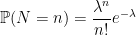
A random variable N has the Poisson distribution with parameter ${\lambda}$ , denoted by ${N\sim{\rm Po}(\lambda)}$ , if it takes values in the set of nonnegative integers and

$\displaystyle {\mathbb P}(N=n)=\frac{\lambda^n}{n!}e^{-\lambda}$

(1)

for each ${n\in{\mathbb Z}_+}$ . The mean and variance of N are both equal to ${\lambda}$ , and the moment generating function can be calculated,

$\displaystyle {\mathbb E}\left[e^{aN}\right] = \exp\left(\lambda(e^a-1)\right),$

which is valid for all ${a\in{\mathbb C}}$ . From this, it can be seen that the sum of independent Poisson random variables with parameters ${\lambda}$ and ${\mu}$ is again Poisson with parameter ${\lambda+\mu}$ . The Poisson distribution occurs as a limit of binomial distributions. The binomial distribution with success probability p and m trials, denoted by ${{\rm Bin}(m,p)}$ , is the sum of m independent ${\{0,1\}}$ -valued random variables each with probability p of being 1. Explicitly, if ${N\sim{\rm Bin}(m,p)}$ then

$\displaystyle {\mathbb P}(N=n)=\frac{m!}{n!(m-n)!}p^n(1-p)^{m-n}.$

In the limit as ${m\rightarrow\infty}$ and ${p\rightarrow 0}$ such that ${mp\rightarrow\lambda}$ , it can be verified that this tends to the Poisson distribution (1) with parameter ${\lambda}$ .

Poisson processes are then defined as processes with independent increments and Poisson distributed marginals, as follows.

Definition 1 A Poisson process X of rate ${\lambda\ge0}$ is a cadlag process with ${X_0=0}$ and ${X_t-X_s\sim{\rm Po}(\lambda(t-s))}$ independently of ${\{X_u\colon u\le s\}}$ for all ${s\le t}$ .

An immediate consequence of this definition is that, if X and Y are independent Poisson processes of rates ${\lambda}$ and ${\mu}$ respectively, then their sum ${X+Y}$ is also Poisson with rate ${\lambda+\mu}$ . Continue reading “Poisson Processes” →

Continuous Processes with Independent Increments

A stochastic process X is said to have independent increments if ${X_t-X_s}$ is independent of ${\{X_u\}_{u\le s}}$ for all ${s\le t}$ . For example, standard Brownian motion is a continuous process with independent increments. Brownian motion also has stationary increments, meaning that the distribution of ${X_{t+s}-X_t}$ does not depend on t. In fact, as I will show in this post, up to a scaling factor and linear drift term, Brownian motion is the only such process. That is, any continuous real-valued process X with stationary independent increments can be written as

$\displaystyle X_t = X_0 + b t + \sigma B_t$

(1)

for a Brownian motion B and constants ${b,\sigma}$ . This is not so surprising in light of the central limit theorem. The increment of a process across an interval [s,t] can be viewed as the sum of its increments over a large number of small time intervals partitioning [s,t]. If these terms are independent with relatively small variance, then the central limit theorem does suggest that their sum should be normally distributed. Together with the previous posts on Lévy’s characterization and stochastic time changes, this provides yet more justification for the ubiquitous position of Brownian motion in the theory of continuous-time processes. Consider, for example, stochastic differential equations such as the Langevin equation. The natural requirements for the stochastic driving term in such equations is that they be continuous with stationary independent increments and, therefore, can be written in terms of Brownian motion.

The definition of standard Brownian motion extends naturally to multidimensional processes and general covariance matrices. A standard d-dimensional Brownian motion ${B=(B^1,\ldots,B^d)}$ is a continuous process with stationary independent increments such that ${B_t}$ has the ${N(0,tI)}$ distribution for all ${t\ge 0}$ . That is, ${B_t}$ is joint normal with zero mean and covariance matrix tI. From this definition, ${B_t-B_s}$ has the ${N(0,(t-s)I)}$ distribution independently of ${\{B_u\colon u\le s\}}$ for all ${s\le t}$ . This definition can be further generalized. Given any ${b\in{\mathbb R}^d}$ and positive semidefinite ${\Sigma\in{\mathbb R}^{d^2}}$ , we can consider a d-dimensional process X with continuous paths and stationary independent increments such that ${X_t}$ has the ${N(tb,t\Sigma)}$ distribution for all ${t\ge 0}$ . Here, ${b}$ is the drift of the process and ${\Sigma}$ is the `instantaneous covariance matrix’. Such processes are sometimes referred to as ${(b,\Sigma)}$ -Brownian motions, and all continuous d-dimensional processes starting from zero and with stationary independent increments are of this form.

Theorem 1 Let X be a continuous ${{\mathbb R}^d}$ -valued process with stationary independent increments.

Then, there exist unique ${b\in{\mathbb R}^d}$ and ${\Sigma\in{\mathbb R}^{d^2}}$ such that ${X_t-X_0}$ is a ${(b,\Sigma)}$ -Brownian motion.

Continue reading “Continuous Processes with Independent Increments” →

Failure of Pathwise Integration for FV Processes

Figure 1: A non-pathwise stochastic integral of an FV Process

The motivation for developing a theory of stochastic integration is that many important processes — such as standard Brownian motion — have sample paths which are extraordinarily badly behaved. With probability one, the path of a Brownian motion is nowhere differentiable and has infinite variation over all nonempty time intervals. This rules out the application of the techniques of ordinary calculus. In particular, the Stieltjes integral can be applied with respect to integrators of finite variation, but fails to give a well-defined integral with respect to Brownian motion. The Ito stochastic integral was developed to overcome this difficulty, at the cost both of restricting the integrand to be an adapted process, and the loss of pathwise convergence in the dominated convergence theorem (convergence in probability holds intead).

However, as I demonstrate in this post, the stochastic integral represents a strict generalization of the pathwise Lebesgue-Stieltjes integral even for processes of finite variation. That is, if V has finite variation, then there can still be predictable integrands ${\xi}$ such that the integral ${\int\xi\,dV}$ is undefined as a Lebesgue-Stieltjes integral on the sample paths, but is well-defined in the Ito sense. Continue reading “Failure of Pathwise Integration for FV Processes” →

Stochastic Calculus Examples and Counterexamples

I have been posting my stochastic calculus notes on this blog for some time, and they have now reached a reasonable level of sophistication. The basics of stochastic integration with respect to local martingales and general semimartingales have been introduced from a rigorous mathematical standpoint, and important results such as Ito’s lemma, the Ito isometry, preservation of the local martingale property, and existence of solutions to stochastic differential equations have been covered.

I will now start to also post examples demonstrating results from stochastic calculus, as well as counterexamples showing how the methods can break down when the required conditions are not quite met. As well as knowing precise mathematical statements and understanding how to prove them, I generally feel that it can be just as important to understand the limits of the results and how they can break down. Knowing good counterexamples can help with this. In stochastic calculus, especially, many statements have quite subtle conditions which, if dropped, invalidate the whole result. In particular, measurability and integrability conditions are often required in subtle ways. Knowing some counterexamples can help to understand these issues. Continue reading “Stochastic Calculus Examples and Counterexamples” →

	SilverBladeII on Cadlag Modifications
	Anonymous on Spitzer’s Formula
	Anonymous on Spitzer’s Formula
	Anonymous on Brownian Bridges
	Anonymous on Spitzer’s Formula
	Anonymous on Spitzer’s Formula
	Anonymous on Spitzer’s Formula
	Anonymous on Spitzer’s Formula
	Anonymous on Spitzer’s Formula
	Anonymous on Spitzer’s Formula