The drawdown of a stochastic process is the amount that it has dropped since it last hit its maximum value so far. For process X with running maximum X∗t = sups ≤ tXs, the drawdown is thus X∗t – Xt, which is a nonnegative process. This is as in figure 1 below.
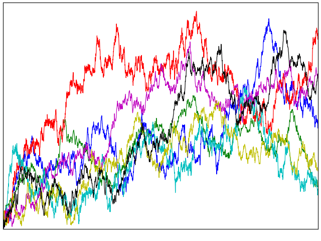
Figure 1: Brownian motion and its drawdown process
For a process X started from zero, its maximum and drawdown can be written as X∗t – X0 and X∗t – Xt. Reversing the process in time across the interval [0, t] will exchange these values. So, reversing in time and translating so that it still starts from zero will exchange the maximum value and the drawdown. Specifically, write
for time index 0 ≤ s ≤ t. The maximum of Y is equal to the drawdown of X,
If X is standard Brownian motion then so is Y, since the independent normal increments property for Y follows from that of X. As already stated, the maximum Y∗t = X∗t – Xt has the same distribution as the absolute value |Yt|= |Xt|. So, the drawdown has the same distribution as the absolute value at each time.
Lemma 1 If X is standard Brownian motion, then X∗t – Xt has the same distribution as |Xt| at each time t ≥ 0.
The distribution of a standard Brownian motion X at a positive time t is, by definition, centered normal with variance t. What can we say about its maximum value up until the time? This is X∗t = sups ≤ tXs, and is clearly nonnegative and at least as big as Xt. To be more precise, consider the probability that the maximum is greater than a fixed positive value a. Such problems will be familiar to anyone who has looked at pricing of financial derivatives such as barrier options, where the payoff of a trade depends on whether the maximum or minimum of an asset price has crossed a specified barrier level.
This can be computed with the aid of a symmetry argument commonly referred to as the reflection principle. The idea is that, if we reflect the Brownian motion when it first hits a level, then the resulting process is also a Brownian motion. The first time at which X hits level a is τ = inf{t ≥ 0: Xt ≥ a}, which is a stopping time. Reflecting the process about this level at all times after τ gives a new process
Figure 1: Reflecting Brownian motion when it hits level a.
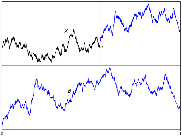
Having previously looked at Brownian bridges and excursions, I now turn to a third kind of process which can be constructed either as a conditioned Brownian motion or by extracting a segment from Brownian motion sample paths. Specifically, the Brownian meander, which is a Brownian motion conditioned to be positive over a unit time interval. Since this requires conditioning on a zero probability event, care must be taken. Instead, it is cleaner to start with an alternative definition by appropriately scaling a segment of a Brownian motion.
For a fixed positive times T, consider the last time σ before T at which a Brownian motion X is equal to zero,
(1)
On interval [σ, T], the path of X will start from 0 and then be either strictly positive or strictly negative, and we may as well restrict to the positive case by taking absolute values. Scaling invariance says that c-1/2Xct is itself a standard Brownian motion for any positive constant c. So, scaling the path of X on [σ, 1] to the unit interval defines a process
(2)
over 0 ≤ t ≤ 1; This starts from zero and is strictly positive at all other times.
Figure 2: Constructing a Brownian meander
Scaling invariance shows that the law of the process B does not depend on the choice of fixed time T The only remaining ambiguity is in the choice of the fixed time T.
Lemma 1 The distribution of B defined by (2) does not depend on the choice of the time T > 0.
Proof: Consider any other fixed positive time T̃, and use the construction above with T̃, σ̃, B̃ in place of T, σ, B respectively. We need to show that B̃ and B have the same distribution. Using the scaling factor S = T̃/T, then X′t = S-1/2XtS is a standard Brownian motion. Also, σ′= σ̃/S is the last time before T at which X′ is zero. So,
has the same distribution as B. ⬜
This leads to the definition used here for Brownian meanders.
Definition 2 A continuous process {Bt}t ∈ [0, 1] is a Brownian meander if and only it has the same distribution as (2) for a standard Brownian motion X and fixed time T > 0.
In fact, there are various alternative — but equivalent — ways in which Brownian excursions can be defined and constructed.
As a scaled segment of a Brownian motion before a time T and after it last hits 0. This is definition 2.
As a Brownian motion conditioned on being positive. See theorem 4 below.
As a segment of a Brownian excursion. See lemma 5.
As the path of a standard Brownian motion starting from its minimum, in either the forwards or backwards direction. See theorem 6.
As a Markov process with specified transition probabilities. See theorem 9 below.