In this post I attempt to give a rigorous definition of integration with respect to Brownian motion (as introduced by Itô in 1944), while keeping it as concise as possible. The stochastic integral can also be defined for a much more general class of processes called semimartingales. However, as Brownian motion is such an important special case which can be handled directly, I start with this as the subject of this post. If  is a standard Brownian motion defined on a probability space
  and
and  is a stochastic process, the aim is to define the integral
 |
(1) |
In ordinary calculus, this can be approximated by Riemann sums, which converge for continuous integrands whenever the integrator  is of finite variation. This leads to the Riemann-Stietjes integral and, generalizing to measurable integrands, the Lebesgue-Stieltjes integral. Unfortunately this method does not work for Brownian motion which, as discussed in my previous post, has infinite variation over all nontrivial compact intervals.
The standard approach is to start by writing out the integral explicitly for piecewise constant integrands. If there are times  such that
  for each
  then the integral is given by the summation,
 |
(2) |
We could try to extend to more general integrands by approximating by piecewise constant processes but, as mentioned above, Brownian motion has infinite variation paths and this will diverge in general.
Fortunately, when working with random processes, there are a couple of observations which improve the chances of being able to consistently define the integral. They are
- The integral is not a single real number, but is instead a random variable defined on the probability space. It therefore only has to be defined up to a set of zero probability and not on every possible path of .
- Rather than requiring limits of integrals to converge for each path of (e.g., dominated convergence), the much weaker convergence in probability can be used.
These observations are still not enough, and the main insight is to only look at integrands which are adapted. That is, the value of  can only depend on through its values at prior times. This condition is met in most situations where we need to use stochastic calculus, such as with (forward) stochastic differential equations. To make this rigorous, for each time
  let
let  be the sigma-algebra generated by
  for all
  . This is a filtration (
 for ), and
  is referred to as a filtered probability space. Then,
  is adapted if is -measurable for all times
  . Piecewise constant and left-continuous processes, such as in (2), which are also adapted are commonly referred to as simple processes.
However, as with standard Lebesgue integration, we must further impose a measurability property. A stochastic process can be viewed as a map from the product space  to the real numbers, given by
  . It is said to be jointly measurable if it is measurable with respect to the product sigma-algebra
  , where
  refers to the Borel sigma-algebra. Finally, it is called progressively measurable, or just progressive, if its restriction to
 ![{[0,t]\times\Omega}](https://s0.wp.com/latex.php?latex=%7B%5B0%2Ct%5D%5Ctimes%5COmega%7D&bg=ffffff&fg=000000&s=0&c=20201002) is
is ![{\mathcal{B}([0,t])\otimes\mathcal{F}_t}](https://s0.wp.com/latex.php?latex=%7B%5Cmathcal%7BB%7D%28%5B0%2Ct%5D%29%5Cotimes%5Cmathcal%7BF%7D_t%7D&bg=ffffff&fg=000000&s=0&c=20201002) -measurable for each positive time . It is easily shown that progressively measurable processes are adapted, and the simple processes introduced above are progressive.
-measurable for each positive time . It is easily shown that progressively measurable processes are adapted, and the simple processes introduced above are progressive.
With these definitions, the stochastic integral of a progressively measurable process with respect to Brownian motion is defined whenever  almost surely (that is, with probability one). The integral (1) is a random variable, defined uniquely up to sets of zero probability by the following two properties.
Continue reading “Integrating with respect to Brownian motion” →
![{U\equiv\exp(X-\frac{1}{2}{\rm Var}(X)-{\mathbb E}[X])}](https://s0.wp.com/latex.php?latex=%7BU%5Cequiv%5Cexp%28X-%5Cfrac%7B1%7D%7B2%7D%7B%5Crm+Var%7D%28X%29-%7B%5Cmathbb+E%7D%5BX%5D%29%7D&bg=ffffff&fg=000000&s=0&c=20201002)

![{{\mathbb Q}(A)={\mathbb E}[1_AU]}](https://s0.wp.com/latex.php?latex=%7B%7B%5Cmathbb+Q%7D%28A%29%3D%7B%5Cmathbb+E%7D%5B1_AU%5D%7D&bg=ffffff&fg=000000&s=0&c=20201002)


![{{\mathbb E}_{\mathbb Q}[Z]={\mathbb E}[UZ]}](https://s0.wp.com/latex.php?latex=%7B%7B%5Cmathbb+E%7D_%7B%5Cmathbb+Q%7D%5BZ%5D%3D%7B%5Cmathbb+E%7D%5BUZ%5D%7D&bg=ffffff&fg=000000&s=0&c=20201002)

![\displaystyle {\mathbb E}_{\mathbb Q}\left[f(Y)\right]={\mathbb E}\left[f\left(Y+{\rm Cov}(X,Y)\right)\right],](https://s0.wp.com/latex.php?latex=%5Cdisplaystyle++%7B%5Cmathbb+E%7D_%7B%5Cmathbb+Q%7D%5Cleft%5Bf%28Y%29%5Cright%5D%3D%7B%5Cmathbb+E%7D%5Cleft%5Bf%5Cleft%28Y%2B%7B%5Crm+Cov%7D%28X%2CY%29%5Cright%29%5Cright%5D%2C+&bg=ffffff&fg=000000&s=0&c=20201002)


![{[0,T]}](https://s0.wp.com/latex.php?latex=%7B%5B0%2CT%5D%7D&bg=ffffff&fg=000000&s=0&c=20201002)
 will be normal with mean zero and variance c(t–s) for times
  . So, scaling the time axis of Brownian motion B to get the new process
  just results in another Brownian motion scaled by the factor
  .
.
 and Brownian motion B on the
  is a deterministic process, not depending on the underlying probability space
  . If
. If  is finite for each
  then the stochastic integral
 has variance
 ![\displaystyle \setlength\arraycolsep{2pt} \begin{array}{rl} \displaystyle{\mathbb E}\left[\left(\int_s^t\xi\,dB\right)^2\right]&\displaystyle={\mathbb E}\left[\int_s^t\xi^2_u\,du\right]\smallskip\\ &\displaystyle=\theta(t)-\theta(s)\smallskip\\ &\displaystyle={\mathbb E}\left[(B_{\theta(t)}-B_{\theta(s)})^2\right]. \end{array}](https://s0.wp.com/latex.php?latex=%5Cdisplaystyle++%5Csetlength%5Carraycolsep%7B2pt%7D+%5Cbegin%7Barray%7D%7Brl%7D+%5Cdisplaystyle%7B%5Cmathbb+E%7D%5Cleft%5B%5Cleft%28%5Cint_s%5Et%5Cxi%5C%2CdB%5Cright%29%5E2%5Cright%5D%26%5Cdisplaystyle%3D%7B%5Cmathbb+E%7D%5Cleft%5B%5Cint_s%5Et%5Cxi%5E2_u%5C%2Cdu%5Cright%5D%5Csmallskip%5C%5C+%26%5Cdisplaystyle%3D%5Ctheta%28t%29-%5Ctheta%28s%29%5Csmallskip%5C%5C+%26%5Cdisplaystyle%3D%7B%5Cmathbb+E%7D%5Cleft%5B%28B_%7B%5Ctheta%28t%29%7D-B_%7B%5Ctheta%28s%29%7D%29%5E2%5Cright%5D.+%5Cend%7Barray%7D+&bg=ffffff&fg=000000&s=0&c=20201002)
 has the same distribution as the time-changed Brownian motion
  .
. , is defined to be a real-valued process satisfying the following properties.
 .
. is normally distributed with mean 0 and variance t–s independently of
  , for any
  for each
 ![{[B]_t=t}](https://s0.wp.com/latex.php?latex=%7B%5BB%5D_t%3Dt%7D&bg=ffffff&fg=000000&s=0&c=20201002) . An incredibly useful result is that the converse statement holds. That is, Brownian motion is the only
. An incredibly useful result is that the converse statement holds. That is, Brownian motion is the only  . Then, the following are equivalent.
  is a local martingale.
 ![{[X]_t=t}](https://s0.wp.com/latex.php?latex=%7B%5BX%5D_t%3Dt%7D&bg=ffffff&fg=000000&s=0&c=20201002) .
.  can be written as
  . The following identity is easily verified,
![{[0,t]}](https://s0.wp.com/latex.php?latex=%7B%5B0%2Ct%5D%7D&bg=ffffff&fg=000000&s=0&c=20201002) into
into  equal parts. That is, set
  for
for  . Then, using
  and summing equation (
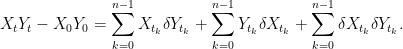
 , and therefore is of order
  . This vanishes in the limit
  , leading to the integration by parts formula
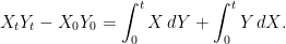
 are
are  are normal random variables with standard deviation
  . It follows that the final term on the right hand side of (
 .
.  and
and  tends to zero in probability as