Feller Processes

George Lowther Special Processes, Stochastic Calculus Notes 14 July 1015 June 20

The definition of Markov processes, as given in the previous post, is much too general for many applications. However, many of the processes which we study also satisfy the much stronger Feller property. This includes Brownian motion, Poisson processes, Lévy processes and Bessel processes, all of which are considered in these notes. Once it is known that a process is Feller, many useful properties follow such as, the existence of cadlag modifications, the strong Markov property, quasi-left-continuity and right-continuity of the filtration. In this post I give the definition of Feller processes and prove the existence of cadlag modifications, leaving the further properties until the next post.

The definition of Feller processes involves putting continuity constraints on the transition function, for which it is necessary to restrict attention to processes lying in a topological space ${(E,\mathcal{T}_E)}$ . It will be assumed that E is locally compact, Hausdorff, and has a countable base (lccb, for short). Such spaces always possess a countable collection of nonvanishing continuous functions ${f\colon E\rightarrow{\mathbb R}}$ which separate the points of E and which, by Lemma 6 below, helps us construct cadlag modifications. Lccb spaces include many of the topological spaces which we may want to consider, such as ${{\mathbb R}^n}$ , topological manifolds and, indeed, any open or closed subset of another lccb space. Such spaces are always Polish spaces, although the converse does not hold (a Polish space need not be locally compact).

Given a topological space E, ${C_0(E)}$ denotes the continuous real-valued functions vanishing at infinity. That is, ${f\colon E\rightarrow{\mathbb R}}$ is in ${C_0(E)}$ if it is continuous and, for any ${\epsilon>0}$ , the set ${\{x\colon \vert f(x)\vert\ge\epsilon\}}$ is compact. Equivalently, its extension to the one-point compactification ${E^*=E\cup\{\infty\}}$ of E given by ${f(\infty)=0}$ is continuous. The set ${C_0(E)}$ is a Banach space under the uniform norm,

$\displaystyle \Vert f\Vert\equiv\sup_{x\in E}\vert f(x)\vert.$

We can now state the general definition of Feller transition functions and processes. A topological space ${(E,\mathcal{T}_E)}$ is also regarded as a measurable space by equipping it with its Borel sigma algebra ${\mathcal{B}(E)=\sigma(\mathcal{T})}$ , so it makes sense to talk of transition probabilities and functions on E.

Definition 1 Let E be an lccb space. Then, a transition function ${\{P_t\}_{t\ge 0}}$ is Feller if, for all ${f\in C_0(E)}$ ,

${P_tf\in C_0(E)}$ .
${t\mapsto P_tf}$ is continuous with respect to the norm topology on ${C_0(E)}$ .
${P_0f=f}$ .

A Markov process X whose transition function is Feller is a Feller process.

Note: Feller processes, as defined here, are sometimes referred to as Feller-Dynkin processes (and similarly for Feller transition functions). The term Feller process is sometimes used to refer to the more general class of processes obtained by replacing ${C_0(E)}$ by the space ${C_b(E)}$ of continuous bounded functions in the definition above. I am following the terminology used by Revuz and Yor (Continuous Martingales and Brownian Motion).

The first condition says that, if X is a Feller process and ${s<t}$ then, the conditional distribution of ${X_t}$ depends on ${X_s}$ in a continuous sense. Also, as ${P_tf\in C_0(E)}$ vanishes at infinity, if S is a compact subset of E, then the probability that ${X_t\in S}$ will vanish conditional on ${X_s}$ being far away. That is, we can find compact sets ${S^\prime}$ such that ${{\mathbb P}(X_t\in S\;\vert X_s\not\in S^\prime)}$ is as small as we like.

Examples of Feller processes include,

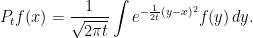
standard Brownian motion, with the transition function
$\displaystyle P_tf(x)=\frac{1}{\sqrt{2\pi t}}\int e^{-\frac{1}{2t}(y-x)^2}f(y)\,dy.$
Poisson processes of rate ${\lambda}$ , with the transition function
$\displaystyle P_tf(x)=\sum_{n=0}^\infty\frac{\lambda^nt^n}{n!}e^{-\lambda t}f(x+n).$

More generally, as we will see in a later post, all ${{\mathbb R}^n}$ -valued processes with stationary independent increments (i.e., Lévy processes) are Feller. In fact, all processes which are continuous in probability and have independent increments, even if they are not stationary, have a Feller space-time process ${(t,X_t)}$ .

Another situation in which Feller processes arise is from stochastic differential equations. Consider the SDE,

$\displaystyle dX^i_t=\sum_{j=1}^ma_{ij}(X_t)\,dB_t^j+b_i(X_t)\,dt,$

( ${i=1,\ldots,n}$ ) for an n-dimensional process X, an m-dimensional Brownian motion B, and Lipschitz-continuous functions ${a_{ij},b\colon{\mathbb R}^n\rightarrow{\mathbb R}}$ . As previously shown, such SDEs have a unique solution for any initial value ${X_0=x}$ . We can then define ${P_t(x,\cdot)}$ to be the distribution of ${X_t}$ , in which case X is Markov with transition function ${\{P_t\}_{t\ge0}}$ . By continuity of solutions with respect to the initial value x, it can be seen that ${P_tf}$ will be continuous for ${f\in C_0({\mathbb R}^n)}$ . Next, as the coefficients are Lipschitz, they cannot grow any faster then linearly as ${\Vert x\Vert\rightarrow\infty}$ . From this, it can be shown that, by making ${x}$ large, the probability of ${X_t}$ being in some fixed bounded region can be made as small as possible (this can be proven using a similar method as showing that SDEs with linearly bounded coefficients cannot explode). So, ${P_tf\in C_0({\mathbb R}^n)}$ . Furthermore, continuity of such processes implies that ${P_tf(x)}$ will be a continuous function of t which, as we will show, implies that ${\{P_t\}}$ is a Feller transition function.

The second condition of Definition 1, that ${t\mapsto P_tf}$ is continuous under the norm topology, can sometimes be quite tricky to prove. Fortunately, this is not necessary, as it turns out to be equivalent to a seemingly much weaker condition. That is, as stated in Theorem 7 below, it is enough to show that ${P_tf(x)\rightarrow f(x)}$ as ${t\rightarrow 0}$ , for each ${f\in C_0(E)}$ . In particular, in the examples of Feller processes mentioned above, this property is implied by continuity in probability.

Definition 1 generalizes to sub-Markovian transition functions, where it is not assumed that ${P_t(x,\cdot)}$ are probability measures. Instead, the inequality ${P_t(x,E)\le1}$ imposed, so the probabilities could sum to less than one. As with general sub-Markovian transition functions, it is possible to extend the state space by adding a cemetery or coffin state ${\Delta}$ , and setting ${E_\Delta=E\cup\{\infty\}}$ . The open sets defining the topology on this space consists of the subsets ${A\subseteq E_\Delta}$ such that ${A\setminus\{\Delta\}}$ is open in E. Equivalently, ${\Delta}$ is an isolated point and the subspace topology on E agrees with the original topology. Then, ${E_\Delta}$ is also an lccb space and defining ${P^\Delta_t}$ as before,

$\displaystyle P_t^\Delta f(x)=\begin{cases} P_tf\vert_E(x)+(1-P_t(x,E))f(\Delta),&\textrm{if }x\in E,\\ f(\Delta),&\textrm{if }x=\Delta, \end{cases}$

(1)

gives a Feller transition function on ${E_\Delta}$ describing a process which can jump to the state ${\Delta}$ , and remain there.

The definition of Feller transition functions can be considered in the more general context of continuous linear semigroups on the Banach space ${C_0(E)}$ . If ${\mu}$ is a probability measure on E then its integral, ${\mu(f)\equiv\int f\,d\mu}$ defines a linear map from ${C_0(E)}$ to ${{\mathbb R}}$ . The converse is given by the Riesz representation theorem, which I state here without proof.

Theorem 2 (Riesz-Markov) Let E be a locally compact Hausdorff space and ${L\colon C_0(E)\rightarrow{\mathbb R}}$ be a continuous linear functional. Then, there is a unique regular (finite signed) measure ${\mu}$ on E such that ${Lf=\mu(f)}$ . Furthermore, ${\Vert L\Vert = \vert\mu\vert(E)}$ .

The condition that ${\mu}$ is regular is not important here, as all finite signed measures on the Borel sigma-algebra are regular in the case of lccb spaces. Then ${\mu}$ is a probability measure if and only if L is positive and ${\Vert L\Vert=1}$ . Similarly, a positive linear function ${L\colon C_0(E)\rightarrow C_0(E)}$ uniquely defines a transition kernel N such that ${Lf=Nf}$ . The property that ${N(x,E)=1}$ , so that N is a transition probability is a bit trickier to state in terms of L. However, the inequality ${\Vert L\Vert\le1}$ is equivalent to ${N(x,E)\le1}$ , allowing us to define sub-Markovian transition functions. A sub-Markovian Feller transition function ${\{P_t\}_{t\ge0}}$ uniquely defines a strongly continuous semigroup of positive linear operators ${\{L_t\}_{t\ge0}}$ on ${C_0(E)}$ such that ${\Vert L_t\Vert\le1}$ , simply by setting ${L_tf=P_tf}$ . Conversely, applying the Riesz representation theorem, every such semigroup arises in this way from a unique sub-Markovian Feller transition function.

The main property of Feller processes, which we concentrate on here, is that they always have cadlag modifications.

Theorem 3 Any Feller process has a cadlag modification.

The proof of this is given below. A consequence is that any Feller transition function ${\{P_t\}}$ can be realized on the space of cadlag functions from ${{\mathbb R}_+}$ to E. This is a big improvement over Theorem 5 of the previous post, which applied to arbitrary transition functions but did not impose any properties on the paths of the process.

Corollary 4 Let E be an lccb space and ${\Omega\subseteq E^{{\mathbb R}_+}}$ be the space of cadlag functions from ${{\mathbb R}_+}$ to E. Denote its coordinate process by ${X_t(\omega)\equiv\omega(t)}$ , let ${\mathcal{F}^0}$ be the sigma-algebra on ${\Omega}$ generated by ${\{X_t\colon t\in{\mathbb R}_+\}}$ and, for each ${t\ge 0}$ , let ${\mathcal{F}^0_t}$ be the sigma-algebra generated by ${\{X_s\colon s\le t\}}$ .

Then, for any Feller transition function ${\{P_t\}}$ and probability measure ${\mu}$ on E, there is a unique probability measure on ${(\Omega,\mathcal{F}^0)}$ with respect to which X is a Feller process with the given transition function and with initial distribution ${X_0\sim\mu}$ .

Proof: By Lemma 3 of the previous post the measure ${{\mathbb P}}$ , if it exists, is unique. We just need to construct one such measure.

Let ${\Omega^\prime=E^{{\mathbb R}_+}}$ with coordinate process ${X^\prime}$ generating the sigma algebra ${\mathcal{F}^\prime}$ so that, by Theorem 5 of the previous post, there is a probability measure ${{\mathbb P}^\prime}$ on ${(\Omega^\prime,\mathcal{F}^\prime)}$ with respect to which ${X^\prime}$ is Markov with the given transition function and initial distribution. Then, by Theorem 3, ${X^\prime}$ has a cadlag modification Y, say. As Y is cadlag, it defines a map ${Y\colon\Omega^\prime\rightarrow\Omega}$ . Let ${{\mathbb P}(A)\equiv{\mathbb P}^\prime(Y^{-1}(A))}$ be the measure induced on ${(\Omega,\mathcal{F}^0)}$ by this map. So X has the same distribution under ${{\mathbb P}}$ as Y does under ${{\mathbb P}^\prime}$ , and hence is Markov with the given transition function and initial distribution. ⬜

We now move on to the proof that Feller processes have cadlag versions. This will be split up into a couple of lemmas, the idea being to show that certain functions of Feller processes are supermartingales and, hence, existence of cadlag modifications for supermartingales can be applied.

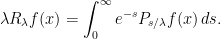
For each ${\lambda>0}$ , the resolvent ${R_\lambda}$ of a transition function ${\{P_t\}_{t\ge 0}}$ on a measurable space ${(E,\mathcal{E})}$ is the kernel defined by

$\displaystyle R_\lambda f(x)=\int_0^\infty e^{-\lambda t}P_tf(x)\,dt,$

(2)

for each bounded measurable ${f\colon E\rightarrow{\mathbb R}}$ . For this to be well-defined, it is only necessary that ${t\mapsto P_t f(x)}$ is measurable, which is true for Feller processes (since it is continuous for ${f\in C_0(E)}$ ). If ${f\in C_0(E)}$ and the transition function ${\{P_t\}}$ is Feller then, using dominated convergence inside the integral in (2), ${R_\lambda f(x_n)\rightarrow R_\lambda f(x)}$ for any sequence ${x_n\rightarrow x}$ and ${R_\lambda f(x_n)\rightarrow 0}$ for ${x_n}$ tending to the point at infinity. So, ${R_\lambda f\in C_0(E)}$ .

The resolvent identity

$\displaystyle R_\lambda R_\mu = R_\mu R_\lambda = \frac{R_\lambda-R_\mu}{\mu-\lambda}$

for ${\lambda\not=\mu}$ follows directly from applying the definition (2) and applying a change of variables. Alternatively, applying the substitution ${s=\lambda t}$ to (2) gives

$\displaystyle \lambda R_\lambda f(x) = \int_0^\infty e^{-s}P_{s/\lambda} f(x)\,ds.$

(3)

In particular, for a Feller transition function, dominated convergence shows that ${\Vert\lambda R_\lambda f-f\Vert\rightarrow 0}$ as ${\lambda\rightarrow\infty}$ for any ${f\in C_0(E)}$ . Also, equation (3) implies that ${\lambda R_\lambda}$ is a transition probability.

The resolvent helps us find functions of the process which are supermartingales.

Lemma 5 Let X be a Markov process taking values in E and with transition function ${\{P_t\}}$ . Then, for any nonnegative, bounded and measurable ${f\colon E\rightarrow{\mathbb R}}$ and ${\lambda>0}$ ,

$\displaystyle M_t\equiv e^{-\lambda t}R_\lambda f(X_t)$

is a supermartingale.

Proof: Expression (2) for the resolvent gives

$\displaystyle \setlength\arraycolsep{2pt} \begin{array}{rl} \displaystyle e^{-\lambda t}P_tR_\lambda f &\displaystyle= \int_0^\infty e^{-\lambda (s+t)}P_{t+s}f\,ds\smallskip\\ &\displaystyle=R_\lambda f - \int_0^t e^{-\lambda s}P_sf\,ds. \end{array}$

(4)

So, if X is Markov with the given transition function and f is nonnegative then,

$\displaystyle P_tR_\lambda f\le e^{\lambda t}R_\lambda f.$

Applying this to the conditional expectation of M,

$\displaystyle \setlength\arraycolsep{2pt} \begin{array}{rl} \displaystyle{\mathbb E}[M_t\;\vert\mathcal{F}_s]&\displaystyle=e^{-\lambda t}{\mathbb E}[R_\lambda f(X_t)\;\vert\mathcal{F}_s] \smallskip\\ &\displaystyle=e^{-\lambda t}P_{t-s}R_\lambda f(X_s)\smallskip\\ &\displaystyle\le e^{-\lambda s}R_\lambda f(X_s)=M_s. \end{array}$

⬜

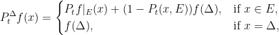
Next, it can be shown that if ${f(X)}$ has a cadlag modification for enough functions ${f\in C_0(E)}$ , then X itself must have a cadlag modification. This does, however, require the state space to be compact. Although Feller processes are defined above for arbitrary lccb spaces, it is always possible to reduce it to the case where E is compact. This can be done by taking the one-point compactification ${E^*=E\cup\{\infty\}}$ of E. Then,

$\displaystyle \tilde P_tf(x)=\begin{cases} P_tf\vert_E(x),&\textrm{if }x\in E,\\ f(\infty),&\textrm{if }x=\infty \end{cases}$

(for bounded measurable ${f\colon E^*\rightarrow{\mathbb R}}$ ) defines a Feller transition function on ${E^*}$ which reduces to ${P_t}$ on E. This describes a process which is either in E behaving according to the transition function ${\{P_t\}}$ , or is fixed at the point at infinity.

Lemma 6 Let ${{\it E}}$ be a compact topological space and ${S=\{f_1,f_2,\ldots\}\subseteq C(E)}$ be a countable sequence of functions separating points in E.

Then, a stochastic process X taking values in E has a cadlag modification if ${f(X)}$ has a cadlag modification for all ${f\in S}$ .

Proof: We first show that a sequence ${x_n}$ in E is convergent if and only if ${f(x_n)}$ converges for every ${f\in S}$ , and that ${x=\lim_{n\rightarrow\infty}x_n}$ is the unique element of E such that ${f(x_n)\rightarrow f(x)}$ for all ${f\in S}$ . By continuity, this is a necessary condition for convergence and for x to be the limit, so we only need to show that it is sufficient. By compactness, every sequence has at least one limit point, and a sequence converges if and only if the limit point is unique. So, suppose that ${f(x_n)}$ converges for all ${f\in S}$ and let ${x,y}$ be limit points of ${x_n}$ . Then, ${f(x)=\lim_nf(x_n)=f(y)}$ and, as S separates points, ${x=y}$ as required. Next, if x is any point satisfying ${f(x_n)\rightarrow f(x)}$ for ${f\in S}$ then, ${f(x)=\lim_nf(x_n)=f(\lim_nx_n)}$ . Since S separates points, we have ${x=\lim_nx_n}$ as promised.

Now suppose that ${f(X)}$ has a cadlag modification ${Y^k}$ , say, for each k. Then, restricting to a set of probability one, ${f_k(X_t)=Y^k_t}$ for all ${k=1,2,\ldots}$ and ${t\in{\mathbb Q}_+}$ . It follows that ${f_k(X_t)}$ , restricted to ${t\in{\mathbb Q}_+}$ , is right-continuous and has left and right limits at all nonnegative reals. By the condition above for convergence in E, ${\{X_t\}_{t\in{\mathbb Q}_+}}$ is also right-continuous with left and right limits everywhere in ${{\mathbb R}_+}$ . So, we can define the cadlag modification

$\displaystyle \hat X_t=\lim_{\substack{s\downarrow t,\\ s\in{\mathbb Q}_+}}X_s.$

⬜

Using Lemma 5 to find functions ${f\in C_0(X)}$ such that ${f(X)}$ has a cadlag modification and applying Lemma 6 to find a cadlag version gives us the proof of Theorem 3.

Proof of Theorem 3: We first prove this in the case where E is compact. Then, for each nonnegative ${f\in C_0(E)}$ , the process ${M_t=e^{-\lambda t}R_\lambda f(X_t)}$ is a supermartingale and, if it is right-continuous in probability, it will have a cadlag modification. In fact, ${g(X_t)}$ is right-continuous in probability for any ${g\in C_0(E)}$ . This follows from the criterion that a sequence ${Y_n}$ of real-valued random variables converges to a limit Y in probability if and only if ${{\mathbb E}[1_Sh(Y_n)]\rightarrow{\mathbb E}[1_Sh(Y)]}$ for each continuous and bounded ${h\colon{\mathbb R}\rightarrow{\mathbb R}}$ and Y-measurable set S. If ${t_n\downarrow t}$ and S is ${g(X_t)}$ -measurable then,

$\displaystyle {\mathbb E}[1_Sh(g(X_{t_n}))]={\mathbb E}[1_SP_{t_n-t}(h\circ g)(X_t)]\rightarrow{\mathbb E}[1_Sh(g(X_t))],$

and ${g(X_{t_n})\rightarrow g(X_t)}$ in probability.

As E is an lccb space, there exists a countable set of nonnegative functions ${S\subseteq C_0(E)}$ separating the points in E. Then, ${R_\lambda f(X)}$ has a cadlag modification and, since ${\lambda R_\lambda f\rightarrow f}$ as ${\lambda\rightarrow\infty}$ , the countable set ${S^\prime=\{R_\lambda f\colon f\in S,\lambda\in{\mathbb N}\}}$ also separates the points of E. By Lemma 6, X has a cadlag modification.

Finally, let us consider the case where E is not compact. Then, letting ${E^*=E\cup\{\infty\}}$ be its one-point compactification, X can also be considered as a Feller process with state space ${E^*}$ . So, we may pass to a cadlag modification taking values in ${E^*}$ , and it only needs to be shown that ${X_t\not=\infty}$ and ${X_{t-}\not=\infty}$ for all t, with probability one. To prove this, choose a strictly positive ${f\in C_0(E)}$ and ${\lambda>0}$ , and consider the submartingale ${M_t=e^{-\lambda t}R_\lambda f(X_t)}$ . The function ${g=R_\lambda f}$ will be strictly positive on E, and can be extended to all of ${E^*}$ by setting ${g(\infty)=0}$ . Letting ${\tau_n}$ be the first time at which ${g(X_t)\le 1/n}$ , we can use optional sampling to get

$\displaystyle {\mathbb E}[1_{\{\tau_n\le t\}}e^{-\lambda t}g(X_t)]\le{\mathbb E}[1_{\{\tau_n\le t\}}e^{-\lambda\tau_n}g(X_{\tau_n})]\le1/n$

for each ${n\in{\mathbb N}}$ and ${t\ge 0}$ . Letting n increase to infinity,

$\displaystyle {\mathbb E}[1_{\{\lim_n\tau_n\le t\}}g(X_t)]=0.$

As ${X_t\in E}$ with probability one, ${g(X_t)}$ is strictly positive and, therefore, ${\lim_n\tau_n>t}$ . As this holds for each t, ${\tau_n\rightarrow\infty}$ almost surely, meaning that ${\inf_{t\le T}g(X_t)}$ is almost surely positive for all T and, hence, ${X_t\not=\infty}$ and ${X_{t-}\not=\infty}$ for all t. ${\Box}$

We now show that it, in the definition of Feller processes, it is not necessary to impose the condition that ${t\mapsto P_tf}$ is continuous under the norm topology, for ${f\in C_0(E)}$ . In fact, the much weaker condition that ${P_tf(x)\rightarrow f(x)}$ as ${t\rightarrow0}$ is enough.

Theorem 7 A transition function ${\{P_t\}_{t\ge 0}}$ on an lccb space E is Feller if and only if, for all ${f\in C_0(E)}$ ,

${P_tf\in C_0(E)}$ for all ${t\ge 0}$ .
${P_tf(x)\rightarrow f(x)}$ as ${t\rightarrow0}$ , for each ${x\in E}$ .

Proof: That these properties are necessary is trivial, so we just prove that they are also sufficient. To show that ${t\mapsto P_t f}$ is norm-continuous, it suffices to prove continuity at 0. In that case, if ${t_n\rightarrow t}$ then,

$\displaystyle \Vert P_{t_n}f-P_t f\Vert = \Vert P_{t_n\wedge t}(P_{\vert t_n-t\vert}f-f)\Vert\le\Vert P_{\vert t_n-t\vert}f-f\Vert\rightarrow0$

as required. Now, letting A be the set of all ${f\in C_0(E)}$ such that ${\Vert P_s f-f\Vert\rightarrow 0}$ as ${s\rightarrow0}$ , the idea is to show that every element of ${C_0(E)}$ is in A. In fact, A is closed under the norm topology. If ${f_n\in A}$ converge uniformly to a limit f then,

$\displaystyle \setlength\arraycolsep{2pt} \begin{array}{rl} \displaystyle\Vert P_s f-f\Vert &\displaystyle\le \Vert P_sf_n-f_n\Vert + \Vert f_n-f\Vert +\Vert P_s(f_n-f)\Vert\smallskip\\ &\displaystyle\le \Vert P_sf_n-f_n\Vert + 2\Vert f_n-f\Vert. \end{array}$

As ${s\rightarrow 0}$ , the right hand side tends to ${2 \Vert f_n-f\Vert}$ which, by choosing n large, can be made as small as we like. So, ${\Vert P_s f-f\Vert}$ tends to 0, and ${f\in A}$ .

To find a sequence in A converging to any given ${f\in C_0(E)}$ , we make use of the resolvent. If ${\lambda>0}$ then, by (4),

$\displaystyle P_t R_\lambda f-R_\lambda f=(e^{\lambda t}-1)R_\lambda f-\int_0^te^{\lambda(t-s)}P_s f\,ds.$

As ${P_t}$ and ${\lambda R_\lambda}$ are transition probabilities, this gives ${\Vert P_t f\Vert\le\Vert f\Vert}$ and ${\Vert \lambda R_\lambda f\Vert\le\Vert f\Vert}$ .

$\displaystyle \setlength\arraycolsep{2pt} \begin{array}{rl} \displaystyle\lambda\Vert P_t R_\lambda f-R_\lambda f\Vert&\displaystyle\le (e^{\lambda t}-1)\Vert f\Vert+\lambda\int_0^te^{\lambda(t-s)}\Vert f\Vert\,ds\smallskip\\ &\displaystyle\le2\Vert f\Vert(e^{\lambda t}-1)\rightarrow 0 \end{array}$

as ${t\rightarrow 0}$ . So, ${R_\lambda f\in A}$ . It only remains to show that ${f}$ can be expressed as the uniform limit of such elements of {\t A}.

Choosing a sequence ${\lambda_n\rightarrow\infty}$ , consider ${\lambda_nR_{\lambda_n}f}$ . By assumption, ${P_tf(x)\rightarrow f(x)}$ as ${t\rightarrow0}$ , for all ${x\in E}$ . Then, applying dominated convergence in the integral in (3) gives ${\lambda_nR_{\lambda_n}f(x)\rightarrow f(x)}$ . This is not quite enough, as we need to find a senquence converging uniformly to ${f}$ . However, Lemma 8 below states that it is possible to improve pointwise convergence to norm convergence just by passing to convex combinations. So, there is a sequence in A converging uniformly to ${f}$ , which must therefore also be in A, as required. ⬜

Finally, the proof of Theorem 7 required the following lemma, which allows us to strengthen the convergence of a series in ${C_0(E)}$ from pointwise to uniform convergence simply by passing to convex combinations. The proof of this is rather non-constructive, relying on the Hahn-Banach theorem for locally convex spaces and the Riesz representation theorem (Theorem 2) to give a proof by contradiction. The notation ${{\rm conv}(S)}$ denotes the set of finite linear combinations of elements of a set S.

Lemma 8 Let E be a locally compact space and ${\{f_n\}_{n=1,2,\ldots}}$ be a uniformly bounded sequence of functions in ${C_0(E)}$ converging pointwise to the limit ${f\in C_0(E)}$ . That is, ${f_n(x)\rightarrow f(x)}$ for each ${x\in E}$ .

Then, there is a sequence ${g_n\in{\rm conv}(\{f_1,f_2,\ldots\})}$ converging uniformly to ${f}$ .

Proof: The result is equivalent to the statement that ${f}$ is in the norm closure S, say, of ${{\rm conv}(\{f_1,f_2,\ldots\})}$ . Suppose that this was not the case. Then, by the Hahn-Banach theorem, there exists a linear and norm-continuous map ${L\colon C_0(E)\rightarrow{\mathbb R}}$ such that ${L(g)\le K<L(f)}$ for some constant K and all ${g\in S}$ . Then, the Riesz representation theorem gives a finite signed measure ${\mu}$ satisfying ${\mu(g)=L(g)}$ for ${g\in C_0(E)}$ . However, using bounded convergence, this leads to the following contradiction,

$\displaystyle L(f)=\mu(f)=\lim_{n\rightarrow\infty}\mu(f_n)=\lim_{n\rightarrow\infty}L(f_n)\le K.$

⬜

Published by George Lowther

View all posts by George Lowther

Published 14 July 1015 June 20

21 thoughts on “Feller Processes”

George Lowther says:

16 July 10 at 11:38 PM

Mik – I moved your comment to the About page, and responded there, as it was not relevant to this post.

Reply
Alekk says:

24 July 10 at 4:15 PM

Dear George, thank you for this great post!

Do you think that it might be possible to include examples of processes that are almost Feller – and see how the properties that you prove in this series of posts break for these almost-feller processes ?

Best
Alekk
ps: any reference except Revuz-Yor and Rogers-Williams ?

Reply
1. George Lowther says:
  
  25 July 10 at 10:13 PM
  
  Good idea! I’ll give some thought towards writing a post on “almost” Feller to show how the properties proven here can fail (i.e., existence of cadlag versions, the strong Markov property, right-continuity of the filtration and quasi-left-continuity).
  The next post is going to be on Bessel processes, which *are* Feller. After that, I am planning on a post demonstrating a simple SDE whose solutions are local martingales but fail to be proper martingales. Coincidentally, they also just fail to be Feller processes but, as they satisfy all the properties I have proven for Feller properties, it doesn’t really give the kind of counterexample you are asking for.
  
  Almost-Feller processes could fit into any of the following categories.
  
  1) P_tf(x) is jointly continuous in t and x but not in C₀(E) for f ∈ C₀(E).
  2) The definition of Feller process is satisfied with C_b(E) in place of C₀(E). The is, P_tf is continuous for bounded continuous f, and t → P_tf is continuous under the uniform norm.
  3) t → P_tf is uniformly continuous for f ∈ C₀(E), but P_tf(x) is not continuous in x.
  4) E is not lccb. Either because is not locally compact or because it does not have a countable base.
  
  Examples satisfying (1) and not having cadlag modifications are easy to construct. Just take something standard like Brownian motion or reflecting Brownian motion and remove the point {0} from the state space. Seems like a bit f a cheat, but I think all examples are like this. They are Feller processes in a larger state space with some points removed.
  
  I think processes in class (2) satisfy all the properties of Feller processes anyway. You can pass to a larger space on which it is Feller (using the Gelfand representation) and then show that it doesn’t hit the additional points in the state space anyway (I think…).
  
  Processes in class (3) are easily constructed which fail the strong Markov property. E.g., consider a real-valued process which either stays at zero or is a Brownian motion. This has transition function
  
  $\displaystyle P_tf(x)=\begin{cases} \displaystyle\frac{1}{\sqrt{2\pi t}}\int e^{-\frac{(x-y)^2}{2t}}f(y)\,dy,&\displaystyle\textrm{if }x\not=0,\\ \displaystyle f(0),&\displaystyle\textrm{if }x=0. \end{cases}$
  
  but fails the strong Markov property at times T with X_T=0. Again, I think all examples are similar to this in that they can be considered as processes on a larger space, but with some points identified. You can also construct examples in a similar way in which the completed filtration is not right-continuous.
  
  I need to think about (4).
  
  Any nice examples you or anyone else know of would be gratefully accepted!
  
  Reply
2. George Lowther says:
  
  25 July 10 at 10:51 PM
  
  For references, I’m not sure what is best. I am mainly working through the subject from the perspective of semimartingales in these notes, rather than getting deeply into Markov process theory. All the results I cover here are included in Revuz-Yor. Checking Kallenberg, Foundations of Modern Probability, I see that it has a chapter on Feller Processes and Semigroups.
  
  Reply
TheBridge says:

9 February 12 at 12:01 PM

Hi George,

I was curious about what are necessary conditions that can ensure that the transform by a fonction $F$ of a Markov (or Feller) Processes ensures that it stays Markov (or Feller).

In particular, for a Markov (or Feller) process defined by an SDE (with coefficients s.t. we have existence and uniqueness), is there necessary conditions that would lead to an explicit calculation (using the coefficients of the SDE or the infinitesimal generator of the process itself and of its transform by $F$ ).

The question comes from the fact that I know a few sufficient conditions, but when those are not fullfiled, I feel it is always a case by case study that determines if yes or no the transformed process is Markovian (or Feller), and no general methodology is applicable.

As asked the question is not really completley “well posed” but an answer with additional assumptions on the process itself would still be interesting.

Best regards

Reply
1. George Lowther says:
  
  22 February 12 at 2:09 AM
  
  Sorry for not responding quicker to this question. I did see it, but didn’t have a good answer immediately. I don’t think that there is a good answer to this though. You can easily construct necessary conditions and sufficent conditions on F, but I don’t think there are any useful conditions which are both necessary and sufficient. So, it does depend on your particular application and I think you are right that requires a case by case study.
  
  Reply
  1. TheBridge says:
    
    24 February 12 at 9:29 AM
    
    Hi George,
    
    Thank’s for your answer indeed the problem seems quite difficult to tackle. But I wonder if it is not linked in some way to Lie Group classification of SDE ( you can take a look at Kozlov article and the references therein : “The Group Classification of a Scalar Stochastic Differential Equation” -JOURNAL OF PHYSICS A: MATHEMATICAL AND THEORETICAL,J. Phys. A: Math. Theor. 43 (2010) 055202 (13pp)).
    
    In particular if the group of transformation preserves the Markov property ( I’m not sure about this) and if it can be showed that only those transforms can do so ( even less sure about this), then there’s might be some hope.
    
    Best regards
    
    Reply
Rutger-Jan Lange says:

23 September 16 at 1:51 AM

Hi there, I really like your blog!

I am an econometrician myself, and I appreciate your blog for the intuition that is not provided by many text books. I am actually writing a paper about optimal stopping in higher dimensions, where I actually use Feller processes. But I’m not an expert. I was hoping perhaps you could help me find a reference for a question, that I believe is possibly relatively simple, but haven’t been able to prove it / find a reference. Any suggestions are greatly appreciated.

If we have a Feller process with an infinitesimal generator $A$ and resolvent $R_\lambda$ , then we have $\lambda R_\lambda f \to f$ uniformly as $\lambda \to \infty$ for any $f \in C_0^0$ . We also have the ‘inverse property’ of the resolvent $R_\lambda (\lambda-A) f= f$ for any $f \in C_0^2$ . Multiplying by $\lambda$ and re-writing this equality, we obtain $\lambda^2 R_\lambda f = \lambda R_\lambda A f + \lambda f$ . This shows that $\lambda^2 R_\lambda f(x) \to 0$ for some $x$ as $\lambda \to \infty$ if and only if $f(x)=0$ and $Af(x)=0$ . This property clearly holds for any $x$ if $f$ is $C_0^2$ .

But now suppose $f$ is only $C^2$ locally in the neighbourhoud of the point $x$ , where we evaluate the limit $\lambda\to\infty$ , but elsewhere it is only $C^0$ . Specifically, in my case, it has a kink on a hyper surface of measure zero. But we evaluate $\lambda^2 R_\lambda f(x)$ away from this hyper surface, i.e. we evaluate the limit where $f(x)=0$ and $A f(x)=0$ . Does the result $\lambda^2 R_\lambda f(x) \to 0$ remain true? I believe it does, perhaps by Dynkin’s formula, since $f$ is $C^2$ in any ball around $x$ . Any ideas to the truth of the statement and/or possible references?

Many thanks & best wishes!

Reply
1. Rutger-Jan Lange says:
  
  23 September 16 at 5:39 AM
  
  PS Perhaps the last sentence of my second paragraph is a bit unclear. I meant to say $\lambda^2 R_\lambda f(x) \to 0$ if and only if $f(x)=0$ as well as $Af(x)=0$ are true at the specific location $x$ (and in its infinitesimal neighbourhood for the derivatives to make sense) where we evaluate the limit. Does this statement remain true if $f(x)$ is only locally $C^2$ , i.e. in a small ball around the location $x$ , where $f$ is identically zero in this ball, such that $f(x)=0$ and $Af(x)=0$ ? (I believe so, but can only find proofs if $f$ is globally $C^2$ and vanishes at infinity, i.e. if $f$ is $C_0^2$ , which doesn’t hold for me.)
  
  Reply
  1. George Lowther says:
    
    28 September 16 at 9:25 PM
    
    Hi. I’m not sure where you would find a precise statement of what you are asking. However, I do have a couple of comments. First, you are using $C^2_0$ where I think you need to be using the domain of A. So, I suppose that you are only considering generators with $C_0^2$ in their domain. Such generators can be expressed as a continuous diffusion term plus a jump term (Revuz & Yor state this in their book, Continuous Martingales and Brownian motion). Your later comment suggests that you are only considering the continuous case (i.e., where you say that Af(x)=0 if f is 0 in a neighbourhood of x). Either way, if f is only $C^2$ in a neighbourhood of x, then Af is strictly speaking not well defined as f is not in the domain of A. However, you can define Af in the $C^2$ region as the non- $C^2$ points will only contribute to the jump component, which does not require smoothness properties. As you say, it then reduces to the case where f is 0 in the neighbourhood of x. I think you just need to show that, in that case, $\lambda AR_\lambda f(x)\to0$ . This certainly looks like it should be true. Or, prove directly that $\lambda^2 R_\lambda f(x)\to0$ which, I think, follows from $Af(x)=0$ .
    
    Btw, I moved your comment to the relevant post.
    
    Reply
  2. George Lowther says:
    
    28 September 16 at 9:32 PM
    
    If $f(x)=0$ and $Af(x)=\lim_{t\to0}(P_tf(x)-f(x))/t$ is well defined, you can use.
    
    $\setlength\arraycolsep{2pt}\begin{array}{rl} \displaystyle\lambda^2 R_\lambda f(x)&\displaystyle=\int_0^\infty\lambda^2e^{-\lambda t}P_tf(x)dt\smallskip\\ &\displaystyle=\int_0^\infty te^{-t} (\lambda/t) (P_{t/\lambda}f(x)-f(x))dt+\lambda f(x)\smallskip\\ &\displaystyle\to \int_0^\infty te^{-t} A f(x)dx=Af(x) \end{array}$
    
    Reply
    1. Rutger-Jan Lange says:
      
      30 September 16 at 11:47 AM
      
      Many thanks! I am indeed considering Feller diffusions processes, i.e. no jump component, for which the domain of $A$ includes (at least) the space of $C_0^2$ functions (indeed as in Revuz and Yor). I should have said for some function $f$ in the domain of $A$ , so I was sloppy. Yes I agree that $\lambda A R_\lambda f(x)\to 0$ looks like it should be true if $f(x)$ is locally identically zero, i.e. in some ball around $x$ of strictly positive radius. To me, it seems irrelevant what happens outside of the ball as long as $f$ remains continuous and bounded everywhere (we could still say the resolvent maps $C_b^0$ to itself, right?). Thanks for the derivation as well (last line should probably have $dt$ rather than $dx$ ?) I will let you know when our paper is ready and mention you in the acknowledgements. If you would be interested in reading the draft, then let me know. It’s about a new (we believe) class of monotone and uniformly converging algorithms for calculating the value function for optimal stopping problems in higher dimensions, which are considered hard because they feature free boundaries, using (global) resolvent/integral methods rather than (local) PDE/finite difference methods. Best wishes, Rutger-Jan
Rutger-Jan Lange says:

30 September 16 at 4:16 PM

I was convinced but now I’m having second thoughts… Again take $f\in C_0^0$ and assume $f(x)=0$ for all $x$ inside some ball $B_R$ of radius $R>0$ centred at some location $\bar{x}$ . Clearly, $\lambda R_\lambda f(x) \to 0$ for any $x \in B_R$ . The question remains whether this implies $A [\lambda (R_\lambda f)](\bar{x}) \to 0$ . While this seems plausible, it is not obvious that the derivatives converge to zero… At least, it is not *generally* true that the derivative converges to zero if the value converges to zero.

Reply
1. George Lowther says:
  
  30 September 16 at 4:25 PM
  
  It is true in the context you ask for. I can provide more details later.
  
  Reply
  1. Anonymous says:
    
    30 September 16 at 5:05 PM
    
    That is all I need, so that would be great!! Curious what your solution is. I intuitively believe it to be true, but that’s not good enough, so many thanks for your help.
    
    Reply
    1. George Lowther says:
      
      30 September 16 at 6:32 PM
      
      Consider the following statements.
      
      i) If $Af(x)\equiv\lim_{t\to0}(P_tf(x)-f(x))/t$ exists for some $x$ And $f\in C_b^0$ then $\lambda AR_\lambda f(x)\to Af(x)$ as $\lambda\to\infty$ .
      ii) If $f\in C_b^0$ is zero in a neighbourhood of $x$ then $Af(x)=0$ .
      
      Combining these gives what you want. For the first, use
      
      $\setlength\arraycolsep{2pt}\begin{array}{rl} \displaystyle \lambda AR_\lambda f(x)&\displaystyle=\int_0^\infty e^{-t}\lambda(P_{t/\lambda}f(x)-f(x))dt \smallskip\\ \displaystyle&\displaystyle\to\int_0^\infty e^{-t} t Af(x)dt = Af(x). \end{array}$
      
      For the second, choose $g\in C^2_0$ with $g\ge\lvert f\rvert$ And $g=0$ in a neighbourhood of $x$ . Then, $\lvert P_tf\rvert\le P_tg$ so,
      
      $\setlength\arraycolsep{2pt}\begin{array}{rl} \displaystyle \lvert P_tf(x)-f(x)\rvert/t&\displaystyle\le(P_tg(x)-g(x))/t \smallskip\\ \displaystyle&\displaystyle\to Ag(x)=0. \end{array}$
Rutger-Jan Lange says:

8 October 16 at 7:41 PM

So I was on travels, but that’s great, thanks! In (ii) you wrote $f \in C_b^0$ and $g \in C_0^2$ , was that intentional? Can we take both in $C_b$ ? To make things easier, suppose $f$ is actually non-negative, so we can take $0 \leq f \leq g$ , with $f\in C_b^0$ and $g\in C_b^2$ and both $f$ and $g$ equal to zero in the neighbourhood of $x$ . Then using your argument we can write $0 \leq \lambda^2 R_\lambda f(x) \leq \lambda^2 R_\lambda g(x) \to 0$ , since $g(x)=f(x)=0$ in the vicinity of $x$ , and we can use all the nice resolvent properties on $g \in C_b^2$ , right?

Reply
1. George Lowther says:
  
  9 October 16 at 11:59 PM
  
  I think I may have got a bit mixed up with the indices there — $f$ was intended to be bounded, measurable, and vanishing at infinity. $g$ is twice continuously differentiable and vanishing at infinity. The argument should generalise to arbitrary bounded measurable $f$ though, with a bit more work.
  
  Reply
Hamilton Bellman says:

31 December 17 at 12:41 AM

Dear George, is a Hawkes process a Feller process?

Reply
Matti Kiiski says:

6 May 18 at 5:18 PM

In Theorem 2 (and Lemma 8), I think you need to assume additionally that the space $E$ is $\sigma$ -compact to be able to conclude that the measure $\mu$ is finite. The measure $\mu$ is in general only locally finite.

Thank you for your amazing blog.

Reply
1. Matti Kiiski says:
  
  6 May 18 at 10:48 PM
  
  Nevermind, the finiteness is indeed guaranteed by the continuity.
  
  Reply

	Harry on Filtrations and Adapted P…
	Anonymous on Analytic Sets
	Daniel on Analytic Sets
	Sid on Martingale Convergence
	northwiz on Preservation of the Local Mart…
	George Lowther on Martingale Convergence
	Sid on Martingale Convergence
	George Lowther on The Burkholder-Davis-Gundy Ine…
	George Lowther on Preservation of the Local Mart…
	northwiz on Preservation of the Local Mart…

Like this:

Related

Published by George Lowther

21 thoughts on “Feller Processes”

Leave a Reply to George Lowther Cancel reply