In these notes, the approach taken to stochastic calculus revolves around stochastic integration and the theory of semimartingales. An alternative starting point would be to consider Markov processes. Although I do not take the second approach, all of the special processes considered in the current section are Markov, so it seems like a good idea to introduce the basic definitions and properties now. In fact, all of the special processes considered (Brownian motion, Poisson processes, Lévy processes, Bessel processes) satisfy the much stronger property of being Feller processes, which I will define in the next post.
Intuitively speaking, a process X is Markov if, given its whole past up until some time s, the future behaviour depends only its state at time s. To make this precise, let us suppose that X takes values in a measurable space and, to denote the past, let be the sigma-algebra generated by . The Markov property then says that, for any times and bounded measurable function , the expected value of conditional on is a function of . Equivalently,
A Poisson process is a continuous-time stochastic process which counts the arrival of randomly occurring events. Commonly cited examples which can be modeled by a Poisson process include radioactive decay of atoms and telephone calls arriving at an exchange, in which the number of events occurring in each consecutive time interval are assumed to be independent. Being piecewise constant, Poisson processes have very simple pathwise properties. However, they are very important to the study of stochastic calculus and, together with Brownian motion, forms one of the building blocks for the much more general class of Lévy processes. I will describe some of their properties in this post.
A random variable N has the Poisson distribution with parameter , denoted by , if it takes values in the set of nonnegative integers and
(1)
for each . The mean and variance of N are both equal to , and the moment generating function can be calculated,
which is valid for all . From this, it can be seen that the sum of independent Poisson random variables with parameters and is again Poisson with parameter . The Poisson distribution occurs as a limit of binomial distributions. The binomial distribution with success probability p and m trials, denoted by , is the sum of m independent -valued random variables each with probability p of being 1. Explicitly, if then
In the limit as and such that , it can be verified that this tends to the Poisson distribution (1) with parameter .
Poisson processes are then defined as processes with independent increments and Poisson distributed marginals, as follows.
Definition 1 A Poisson process X of rate is a cadlag process with and independently of for all .
An immediate consequence of this definition is that, if X and Y are independent Poisson processes of rates and respectively, then their sum is also Poisson with rate . Continue reading “Poisson Processes”→
A stochastic process X is said to have independent increments if is independent of for all . For example, standard Brownian motion is a continuous process with independent increments. Brownian motion also has stationary increments, meaning that the distribution of does not depend on t. In fact, as I will show in this post, up to a scaling factor and linear drift term, Brownian motion is the only such process. That is, any continuous real-valued process X with stationary independent increments can be written as
(1)
for a Brownian motion B and constants . This is not so surprising in light of the central limit theorem. The increment of a process across an interval [s,t] can be viewed as the sum of its increments over a large number of small time intervals partitioning [s,t]. If these terms are independent with relatively small variance, then the central limit theorem does suggest that their sum should be normally distributed. Together with the previous posts on Lévy’s characterization and stochastic time changes, this provides yet more justification for the ubiquitous position of Brownian motion in the theory of continuous-time processes. Consider, for example, stochastic differential equations such as the Langevin equation. The natural requirements for the stochastic driving term in such equations is that they be continuous with stationary independent increments and, therefore, can be written in terms of Brownian motion.
The definition of standard Brownian motion extends naturally to multidimensional processes and general covariance matrices. A standard d-dimensional Brownian motion is a continuous process with stationary independent increments such that has the distribution for all . That is, is joint normal with zero mean and covariance matrix tI. From this definition, has the distribution independently of for all . This definition can be further generalized. Given any and positive semidefinite , we can consider a d-dimensional process X with continuous paths and stationary independent increments such that has the distribution for all . Here, is the drift of the process and is the `instantaneous covariance matrix’. Such processes are sometimes referred to as -Brownian motions, and all continuous d-dimensional processes starting from zero and with stationary independent increments are of this form.
Theorem 1 Let X be a continuous -valued process with stationary independent increments.
Then, there exist unique and such that is a -Brownian motion.
The martingale representation theorem states that any martingale adapted with respect to a Brownian motion can be expressed as a stochastic integral with respect to the same Brownian motion.
Theorem 1 Let B be a standard Brownian motion defined on a probability space and be its natural filtration.
As stochastic integration preserves the local martingale property for continuous processes, this result characterizes the space of all local martingales starting from 0 defined with respect to the filtration generated by a Brownian motion as being precisely the set of stochastic integrals with respect to that Brownian motion. Equivalently, Brownian motion has the predictable representation property. This result is often used in mathematical finance as the statement that the Black-Scholes model is complete. That is, any contingent claim can be exactly replicated by trading in the underlying stock. This does involve some rather large and somewhat unrealistic assumptions on the behaviour of financial markets and ability to trade continuously without incurring additional costs. However, in this post, I will be concerned only with the mathematical statement and proof of the representation theorem.
In more generality, the martingale representation theorem can be stated for a d-dimensional Brownian motion as follows.
Theorem 2 Let be a d-dimensional Brownian motion defined on the filtered probability space, and suppose that is the natural filtration generated by B and .
Then, every -local martingale M can be expressed as
(1)
for predictable processes satisfying , almost surely, for each .
The previous two posts described the behaviour of standard Brownian motion under stochastic changes of time and equivalent changes of measure. I now demonstrate some applications of these ideas to the study of stochastic differential equations (SDEs). Surprisingly strong results can be obtained and, in many cases, it is possible to prove existence and uniqueness of solutions to SDEs without imposing any continuity constraints on the coefficients. This is in contrast to most standard existence and uniqueness results for both ordinary and stochastic differential equations, where conditions such as Lipschitz continuity is required. For example, consider the following SDE for measurable coefficients and a Brownian motion B
(1)
If a is nonzero, is locally integrable and b/a is bounded then we can show that this has weak solutions satisfying uniqueness in law for any specified initial distribution of X. The idea is to start with X being a standard Brownian motion and apply a change of time to obtain a solution to (1) in the case where the drift term b is zero. Then, a Girsanov transformation can be used to change to a measure under which X satisfies the SDE for nonzero drift b. As these steps are invertible, every solution can be obtained from a Brownian motion in this way, which uniquely determines the distribution of X.
A standard example demonstrating the concept of weak solutions and uniqueness in law is provided by Tanaka’s SDE
Girsanov transformations describe how Brownian motion and, more generally, local martingales behave under changes of the underlying probability measure. Let us start with a much simpler identity applying to normal random variables. Suppose that X and are jointly normal random variables defined on a probability space . Then is a positive random variable with expectation 1, and a new measure can be defined by for all sets . Writing for expectation under the new measure, then for all bounded random variables Z. The expectation of a bounded measurable function of Y under the new measure is
(1)
where is the covariance. This is a vector whose i’th component is the covariance . So, Y has the same distribution under as has under . That is, when changing to the new measure, Y remains jointly normal with the same covariance matrix, but its mean increases by . Equation (1) follows from a straightforward calculation of the characteristic function of Y with respect to both and .
Now consider a standard Brownian motion B and fix a time and a constant . Then, for all times , the covariance of and is . Applying (1) to the measure shows that
where is a standard Brownian motion under . Under the new measure, B has gained a constant drift of over the interval . Such transformations are widely applied in finance. For example, in the Black-Scholes model of option pricing it is common to work under a risk-neutral measure, which transforms the drift of a financial asset to be the risk-free rate of return. Girsanov transformations extend this idea to much more general changes of measure, and to arbitrary local martingales. However, as shown below, the strongest results are obtained for Brownian motion which, under a change of measure, just gains a stochastic drift term. Continue reading “Girsanov Transformations”→
From the definition of standard Brownian motionB, given any positive constant c, will be normal with mean zero and variance c(t–s) for times . So, scaling the time axis of Brownian motion B to get the new process just results in another Brownian motion scaled by the factor .
This idea is easily generalized. Consider a measurable function and Brownian motion B on the filtered probability space. So, is a deterministic process, not depending on the underlying probability space . If is finite for each then the stochastic integral exists. Furthermore, X will be a Gaussian process with independent increments. For piecewise constant integrands, this results from the fact that linear combinations of joint normal variables are themselves normal. The case for arbitrary deterministic integrands follows by taking limits. Also, the Ito isometry says that has variance
So, has the same distribution as the time-changed Brownian motion .
Standard Brownian motion, , is defined to be a real-valued process satisfying the following properties.
.
is normally distributed with mean 0 and variance t–s independently of , for any .
B has continuous sample paths.
As always, it only really matters is that these properties hold almost surely. Now, to apply the techniques of stochastic calculus, it is assumed that there is an underlying filtered probability space, which necessitates a further definition; a process B is a Brownian motion on a filtered probability space if in addition to the above properties it is also adapted, so that is -measurable, and is independent of for each . Note that the above condition that is independent of is not explicitly required, as it also follows from the independence from . According to these definitions, a process is a Brownian motion if and only if it is a Brownian motion with respect to its natural filtration.
The property that has zero mean independently of means that Brownian motion is a martingale. Furthermore, we previously calculated its quadratic variation as . An incredibly useful result is that the converse statement holds. That is, Brownian motion is the onlylocal martingale with this quadratic variation. This is known as Lévy’s characterization, and shows that Brownian motion is a particularly general stochastic process, justifying its ubiquitous influence on the study of continuous-time stochastic processes.
Theorem 1 (Lévy’s Characterization of Brownian Motion) Let X be a local martingale with . Then, the following are equivalent.
X is standard Brownian motion on the underlying filtered probability space.
The point in these stochastic calculus notes has been reached where the theory of stochastic integration is sufficiently well developed to apply in a wide range of situations.
Over the next few posts, I will take a break from further development of the general theory. Instead, I look at certain special processes, applying the calculus developed so far and gaining a few examples to motivate further development of the theory.


![\displaystyle {\mathbb E}\left[f(X_t)\mid\mathcal{F}_s\right]={\mathbb E}\left[f(X_t)\mid X_s\right]](https://s0.wp.com/latex.php?latex=%5Cdisplaystyle++%7B%5Cmathbb+E%7D%5Cleft%5Bf%28X_t%29%5Cmid%5Cmathcal%7BF%7D_s%5Cright%5D%3D%7B%5Cmathbb+E%7D%5Cleft%5Bf%28X_t%29%5Cmid+X_s%5Cright%5D+&bg=ffffff&fg=000000&s=0&c=20201002)


 , denoted by
  , if it takes values in the set of nonnegative integers and
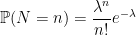
 . The mean and variance of N are both equal to
 ![\displaystyle {\mathbb E}\left[e^{aN}\right] = \exp\left(\lambda(e^a-1)\right),](https://s0.wp.com/latex.php?latex=%5Cdisplaystyle++%7B%5Cmathbb+E%7D%5Cleft%5Be%5E%7BaN%7D%5Cright%5D+%3D+%5Cexp%5Cleft%28%5Clambda%28e%5Ea-1%29%5Cright%29%2C+&bg=ffffff&fg=000000&s=0&c=20201002)
 . From this, it can be seen that the sum of independent Poisson random variables with parameters
  is again Poisson with parameter
  . The Poisson distribution occurs as a limit of
  , is the sum of m independent
  -valued random variables each with probability p of being 1. Explicitly, if
  then
then 
 and
and  such that
  , it can be verified that this tends to the Poisson distribution (
 is a
is a  and
and  independently of
  for all
  is also Poisson with rate
  is independent of
  for all
  does not depend on t. In fact, as I will show in this post, up to a scaling factor and linear drift term, Brownian motion is the only such process. That is, any continuous real-valued process X with stationary independent increments can be written as
 . This is not so surprising in light of the
  is a continuous process with stationary independent increments such that
  has the
  distribution for all
  . That is,
  has the
  distribution independently of
  for all
  and positive semidefinite
  , we can consider a d-dimensional process X with continuous paths and stationary independent increments such that
  has the
  distribution for all
  is the drift of the process and
  is the `instantaneous covariance matrix’. Such processes are sometimes referred to as
  -Brownian motions, and all continuous d-dimensional processes starting from zero and with stationary independent increments are of this form.
 -valued process with stationary independent increments.
 is a
is a  and
and  be its
  –
–
 .
.  , and suppose that
  .
. 

 satisfying
  , almost surely, for each
  .
.  and a Brownian motion B
 is locally integrable and b/a is bounded then we can show that this has weak solutions satisfying uniqueness in law for any specified initial distribution of X. The idea is to start with X being a standard Brownian motion and apply a change of time to obtain a solution to (
 are jointly normal random variables defined on a probability space
 ![{U\equiv\exp(X-\frac{1}{2}{\rm Var}(X)-{\mathbb E}[X])}](https://s0.wp.com/latex.php?latex=%7BU%5Cequiv%5Cexp%28X-%5Cfrac%7B1%7D%7B2%7D%7B%5Crm+Var%7D%28X%29-%7B%5Cmathbb+E%7D%5BX%5D%29%7D&bg=ffffff&fg=000000&s=0&c=20201002) is a positive random variable with expectation 1, and a new measure
is a positive random variable with expectation 1, and a new measure  can be defined by
 ![{{\mathbb Q}(A)={\mathbb E}[1_AU]}](https://s0.wp.com/latex.php?latex=%7B%7B%5Cmathbb+Q%7D%28A%29%3D%7B%5Cmathbb+E%7D%5B1_AU%5D%7D&bg=ffffff&fg=000000&s=0&c=20201002) for all sets
for all sets  . Writing
  for expectation under the new measure, then
 ![{{\mathbb E}_{\mathbb Q}[Z]={\mathbb E}[UZ]}](https://s0.wp.com/latex.php?latex=%7B%7B%5Cmathbb+E%7D_%7B%5Cmathbb+Q%7D%5BZ%5D%3D%7B%5Cmathbb+E%7D%5BUZ%5D%7D&bg=ffffff&fg=000000&s=0&c=20201002) for all bounded random variables Z. The expectation of a bounded measurable function
for all bounded random variables Z. The expectation of a bounded measurable function  of Y under the new measure is
 ![\displaystyle {\mathbb E}_{\mathbb Q}\left[f(Y)\right]={\mathbb E}\left[f\left(Y+{\rm Cov}(X,Y)\right)\right],](https://s0.wp.com/latex.php?latex=%5Cdisplaystyle++%7B%5Cmathbb+E%7D_%7B%5Cmathbb+Q%7D%5Cleft%5Bf%28Y%29%5Cright%5D%3D%7B%5Cmathbb+E%7D%5Cleft%5Bf%5Cleft%28Y%2B%7B%5Crm+Cov%7D%28X%2CY%29%5Cright%29%5Cright%5D%2C+&bg=ffffff&fg=000000&s=0&c=20201002)
 is the covariance. This is a vector whose i’th component is the covariance
  . So, Y has the same distribution under
  as
as  has under
  . That is, when changing to the new measure, Y remains jointly normal with the same covariance matrix, but its mean increases by
  and a constant
  is
is  . Applying (
 shows that
 is a standard Brownian motion under
 ![{[0,T]}](https://s0.wp.com/latex.php?latex=%7B%5B0%2CT%5D%7D&bg=ffffff&fg=000000&s=0&c=20201002) . Such transformations are widely applied in finance. For example, in the Black-Scholes model of option pricing it is common to work under a risk-neutral measure, which transforms the drift of a financial asset to be the risk-free rate of return. Girsanov transformations extend this idea to much more general changes of measure, and to arbitrary local martingales. However,
. Such transformations are widely applied in finance. For example, in the Black-Scholes model of option pricing it is common to work under a risk-neutral measure, which transforms the drift of a financial asset to be the risk-free rate of return. Girsanov transformations extend this idea to much more general changes of measure, and to arbitrary local martingales. However,  will be normal with mean zero and variance c(t–s) for times
  . So, scaling the time axis of Brownian motion B to get the new process
  just results in another Brownian motion scaled by the factor
  .
.
 and Brownian motion B on the
  . If
. If  is finite for each
  then the stochastic integral
![\displaystyle \setlength\arraycolsep{2pt} \begin{array}{rl} \displaystyle{\mathbb E}\left[\left(\int_s^t\xi\,dB\right)^2\right]&\displaystyle={\mathbb E}\left[\int_s^t\xi^2_u\,du\right]\smallskip\\ &\displaystyle=\theta(t)-\theta(s)\smallskip\\ &\displaystyle={\mathbb E}\left[(B_{\theta(t)}-B_{\theta(s)})^2\right]. \end{array}](https://s0.wp.com/latex.php?latex=%5Cdisplaystyle++%5Csetlength%5Carraycolsep%7B2pt%7D+%5Cbegin%7Barray%7D%7Brl%7D+%5Cdisplaystyle%7B%5Cmathbb+E%7D%5Cleft%5B%5Cleft%28%5Cint_s%5Et%5Cxi%5C%2CdB%5Cright%29%5E2%5Cright%5D%26%5Cdisplaystyle%3D%7B%5Cmathbb+E%7D%5Cleft%5B%5Cint_s%5Et%5Cxi%5E2_u%5C%2Cdu%5Cright%5D%5Csmallskip%5C%5C+%26%5Cdisplaystyle%3D%5Ctheta%28t%29-%5Ctheta%28s%29%5Csmallskip%5C%5C+%26%5Cdisplaystyle%3D%7B%5Cmathbb+E%7D%5Cleft%5B%28B_%7B%5Ctheta%28t%29%7D-B_%7B%5Ctheta%28s%29%7D%29%5E2%5Cright%5D.+%5Cend%7Barray%7D+&bg=ffffff&fg=000000&s=0&c=20201002)
 has the same distribution as the time-changed Brownian motion
  .
. , is defined to be a real-valued process satisfying the following properties.
 .
.![{[B]_t=t}](https://s0.wp.com/latex.php?latex=%7B%5BB%5D_t%3Dt%7D&bg=ffffff&fg=000000&s=0&c=20201002) . An incredibly useful result is that the converse statement holds. That is, Brownian motion is the only
. An incredibly useful result is that the converse statement holds. That is, Brownian motion is the only  is a local martingale.
 ![{[X]_t=t}](https://s0.wp.com/latex.php?latex=%7B%5BX%5D_t%3Dt%7D&bg=ffffff&fg=000000&s=0&c=20201002) .
. 