The martingale representation theorem states that any martingale adapted with respect to a Brownian motion can be expressed as a stochastic integral with respect to the same Brownian motion.
Theorem 1 Let B be a standard Brownian motion defined on a probability space
and
be its natural filtration.
Then, every
–local martingale M can be written as
for a predictable, B-integrable, process
.
As stochastic integration preserves the local martingale property for continuous processes, this result characterizes the space of all local martingales starting from 0 defined with respect to the filtration generated by a Brownian motion as being precisely the set of stochastic integrals with respect to that Brownian motion. Equivalently, Brownian motion has the predictable representation property. This result is often used in mathematical finance as the statement that the Black-Scholes model is complete. That is, any contingent claim can be exactly replicated by trading in the underlying stock. This does involve some rather large and somewhat unrealistic assumptions on the behaviour of financial markets and ability to trade continuously without incurring additional costs. However, in this post, I will be concerned only with the mathematical statement and proof of the representation theorem.
In more generality, the martingale representation theorem can be stated for a d-dimensional Brownian motion as follows.
Theorem 2 Let
be a d-dimensional Brownian motion defined on the filtered probability space
, and suppose that
.
Then, every
(1) for predictable processes
satisfying
, almost surely, for each
.


 and a Brownian motion B
 is locally integrable and b/a is bounded then we can show that this has weak solutions satisfying uniqueness in law for any specified initial distribution of X. The idea is to start with X being a standard Brownian motion and apply a change of time to obtain a solution to (
 are jointly normal random variables defined on a probability space
 ![{U\equiv\exp(X-\frac{1}{2}{\rm Var}(X)-{\mathbb E}[X])}](https://s0.wp.com/latex.php?latex=%7BU%5Cequiv%5Cexp%28X-%5Cfrac%7B1%7D%7B2%7D%7B%5Crm+Var%7D%28X%29-%7B%5Cmathbb+E%7D%5BX%5D%29%7D&bg=ffffff&fg=000000&s=0&c=20201002) is a positive random variable with expectation 1, and a new measure
is a positive random variable with expectation 1, and a new measure  can be defined by
 ![{{\mathbb Q}(A)={\mathbb E}[1_AU]}](https://s0.wp.com/latex.php?latex=%7B%7B%5Cmathbb+Q%7D%28A%29%3D%7B%5Cmathbb+E%7D%5B1_AU%5D%7D&bg=ffffff&fg=000000&s=0&c=20201002) for all sets
for all sets  . Writing
  for expectation under the new measure, then
 ![{{\mathbb E}_{\mathbb Q}[Z]={\mathbb E}[UZ]}](https://s0.wp.com/latex.php?latex=%7B%7B%5Cmathbb+E%7D_%7B%5Cmathbb+Q%7D%5BZ%5D%3D%7B%5Cmathbb+E%7D%5BUZ%5D%7D&bg=ffffff&fg=000000&s=0&c=20201002) for all bounded random variables Z. The expectation of a bounded measurable function
for all bounded random variables Z. The expectation of a bounded measurable function  of Y under the new measure is
 ![\displaystyle {\mathbb E}_{\mathbb Q}\left[f(Y)\right]={\mathbb E}\left[f\left(Y+{\rm Cov}(X,Y)\right)\right],](https://s0.wp.com/latex.php?latex=%5Cdisplaystyle++%7B%5Cmathbb+E%7D_%7B%5Cmathbb+Q%7D%5Cleft%5Bf%28Y%29%5Cright%5D%3D%7B%5Cmathbb+E%7D%5Cleft%5Bf%5Cleft%28Y%2B%7B%5Crm+Cov%7D%28X%2CY%29%5Cright%29%5Cright%5D%2C+&bg=ffffff&fg=000000&s=0&c=20201002)
 is the covariance. This is a vector whose i’th component is the covariance
  . So, Y has the same distribution under
  as
as  has under
  . That is, when changing to the new measure, Y remains jointly normal with the same covariance matrix, but its mean increases by
  and a constant
  . Then, for all times
  , the covariance of
  and
and  is
is 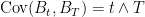 . Applying (
 shows that
 is a standard Brownian motion under
 ![{[0,T]}](https://s0.wp.com/latex.php?latex=%7B%5B0%2CT%5D%7D&bg=ffffff&fg=000000&s=0&c=20201002) . Such transformations are widely applied in finance. For example, in the Black-Scholes model of option pricing it is common to work under a risk-neutral measure, which transforms the drift of a financial asset to be the risk-free rate of return. Girsanov transformations extend this idea to much more general changes of measure, and to arbitrary local martingales. However,
. Such transformations are widely applied in finance. For example, in the Black-Scholes model of option pricing it is common to work under a risk-neutral measure, which transforms the drift of a financial asset to be the risk-free rate of return. Girsanov transformations extend this idea to much more general changes of measure, and to arbitrary local martingales. However,  will be normal with mean zero and variance c(t–s) for times
  . So, scaling the time axis of Brownian motion B to get the new process
  just results in another Brownian motion scaled by the factor
  .
.
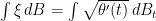
 and Brownian motion B on the
  . If
. If  is finite for each
  then the stochastic integral
 has variance
 ![\displaystyle \setlength\arraycolsep{2pt} \begin{array}{rl} \displaystyle{\mathbb E}\left[\left(\int_s^t\xi\,dB\right)^2\right]&\displaystyle={\mathbb E}\left[\int_s^t\xi^2_u\,du\right]\smallskip\\ &\displaystyle=\theta(t)-\theta(s)\smallskip\\ &\displaystyle={\mathbb E}\left[(B_{\theta(t)}-B_{\theta(s)})^2\right]. \end{array}](https://s0.wp.com/latex.php?latex=%5Cdisplaystyle++%5Csetlength%5Carraycolsep%7B2pt%7D+%5Cbegin%7Barray%7D%7Brl%7D+%5Cdisplaystyle%7B%5Cmathbb+E%7D%5Cleft%5B%5Cleft%28%5Cint_s%5Et%5Cxi%5C%2CdB%5Cright%29%5E2%5Cright%5D%26%5Cdisplaystyle%3D%7B%5Cmathbb+E%7D%5Cleft%5B%5Cint_s%5Et%5Cxi%5E2_u%5C%2Cdu%5Cright%5D%5Csmallskip%5C%5C+%26%5Cdisplaystyle%3D%5Ctheta%28t%29-%5Ctheta%28s%29%5Csmallskip%5C%5C+%26%5Cdisplaystyle%3D%7B%5Cmathbb+E%7D%5Cleft%5B%28B_%7B%5Ctheta%28t%29%7D-B_%7B%5Ctheta%28s%29%7D%29%5E2%5Cright%5D.+%5Cend%7Barray%7D+&bg=ffffff&fg=000000&s=0&c=20201002)
 has the same distribution as the time-changed Brownian motion
  .
. , is defined to be a real-valued process satisfying the following properties.
 .
. is normally distributed with mean 0 and variance t–s independently of
  , for any
  -measurable, and
  for each
 ![{[B]_t=t}](https://s0.wp.com/latex.php?latex=%7B%5BB%5D_t%3Dt%7D&bg=ffffff&fg=000000&s=0&c=20201002) . An incredibly useful result is that the converse statement holds. That is, Brownian motion is the only
. An incredibly useful result is that the converse statement holds. That is, Brownian motion is the only  . Then, the following are equivalent.
  is a local martingale.
 ![{[X]_t=t}](https://s0.wp.com/latex.php?latex=%7B%5BX%5D_t%3Dt%7D&bg=ffffff&fg=000000&s=0&c=20201002) .
.  is its maximum process.
 there exist positive constants
  such that, for all local martingales X with
  , the following inequality holds.
 ![\displaystyle c_p{\mathbb E}\left[ [X]^{p/2}_\tau\right]\le{\mathbb E}\left[(X^*_\tau)^p\right]\le C_p{\mathbb E}\left[ [X]^{p/2}_\tau\right].](https://s0.wp.com/latex.php?latex=%5Cdisplaystyle++c_p%7B%5Cmathbb+E%7D%5Cleft%5B+%5BX%5D%5E%7Bp%2F2%7D_%5Ctau%5Cright%5D%5Cle%7B%5Cmathbb+E%7D%5Cleft%5B%28X%5E%2A_%5Ctau%29%5Ep%5Cright%5D%5Cle+C_p%7B%5Cmathbb+E%7D%5Cleft%5B+%5BX%5D%5E%7Bp%2F2%7D_%5Ctau%5Cright%5D.+&bg=ffffff&fg=000000&s=0&c=20201002)
 .
.  , the theorem can also be stated as follows. The set of all cadlag martingales X starting from zero for which
 ![{{\mathbb E}[(X^*_\infty)^p]}](https://s0.wp.com/latex.php?latex=%7B%7B%5Cmathbb+E%7D%5B%28X%5E%2A_%5Cinfty%29%5Ep%5D%7D&bg=ffffff&fg=000000&s=0&c=20201002) is finite is a vector space, and the BDG inequality states that the norms
is finite is a vector space, and the BDG inequality states that the norms ![{X\mapsto\Vert X^*_\infty\Vert_p={\mathbb E}[(X^*_\infty)^p]^{1/p}}](https://s0.wp.com/latex.php?latex=%7BX%5Cmapsto%5CVert+X%5E%2A_%5Cinfty%5CVert_p%3D%7B%5Cmathbb+E%7D%5B%28X%5E%2A_%5Cinfty%29%5Ep%5D%5E%7B1%2Fp%7D%7D&bg=ffffff&fg=000000&s=0&c=20201002) and
and ![{X\mapsto\Vert[X]^{1/2}_\infty\Vert_p}](https://s0.wp.com/latex.php?latex=%7BX%5Cmapsto%5CVert%5BX%5D%5E%7B1%2F2%7D_%5Cinfty%5CVert_p%7D&bg=ffffff&fg=000000&s=0&c=20201002) are equivalent.
are equivalent. ,
,  . The significance of Theorem
  .
.![{\left[\int\xi\,dX\right]=\int\xi^2\,d[X]}](https://s0.wp.com/latex.php?latex=%7B%5Cleft%5B%5Cint%5Cxi%5C%2CdX%5Cright%5D%3D%5Cint%5Cxi%5E2%5C%2Cd%5BX%5D%7D&bg=ffffff&fg=000000&s=0&c=20201002) . Recall, also, that stochastic integration
. Recall, also, that stochastic integration  -integrable martingales, for
  .
. , so that
 ![{{\mathbb E}[\vert X_t\vert^p]<\infty}](https://s0.wp.com/latex.php?latex=%7B%7B%5Cmathbb+E%7D%5B%5Cvert+X_t%5Cvert%5Ep%5D%3C%5Cinfty%7D&bg=ffffff&fg=000000&s=0&c=20201002) for each t. Then, for any bounded predictable process
for each t. Then, for any bounded predictable process  is also an
  is a continuous local martingale.
 ![\displaystyle \int_0^t\xi^2\,d[X]<\infty](https://s0.wp.com/latex.php?latex=%5Cdisplaystyle++%5Cint_0%5Et%5Cxi%5E2%5C%2Cd%5BX%5D%3C%5Cinfty+&bg=ffffff&fg=000000&s=0&c=20201002)
 is a martingale.
![{X^2-[X]}](https://s0.wp.com/latex.php?latex=%7BX%5E2-%5BX%5D%7D&bg=ffffff&fg=000000&s=0&c=20201002) is a local martingale for all local martingales X.
is a local martingale for all local martingales X. ![\displaystyle XY-[X,Y] = X_0Y_0+\int X_-\,dY+\int Y_-\,dX](https://s0.wp.com/latex.php?latex=%5Cdisplaystyle++XY-%5BX%2CY%5D+%3D+X_0Y_0%2B%5Cint+X_-%5C%2CdY%2B%5Cint+Y_-%5C%2CdX+&bg=ffffff&fg=000000&s=0&c=20201002)
 for some constant K. Then, as
  such that
  converges to
  by
by  if necessary so that, being nonnegative elementary integrals of a submartingale,
  will be submartingales. Also,
  . Recall that a cadlag adapted process X is
  is locally integrable, and all local submartingales are locally integrable. So,
 gives,
 .
. for some
  and
and  .
. 