Recall from the previous post that a cadlag adapted process  is a local martingale if there is a sequence
  of stopping times increasing to infinity such that the stopped processes
  are martingales. Local submartingales and local supermartingales are defined similarly.
An example of a local martingale which is not a martingale is given by the `double-loss’ gambling strategy. Interestingly, in 18th century France, such strategies were known as martingales and is the origin of the mathematical term. Suppose that a gambler is betting sums of money, with even odds, on a simple win/lose game. For example, betting that a coin toss comes up heads. He could bet one dollar on the first toss and, if he loses, double his stake to two dollars for the second toss. If he loses again, then he is down three dollars and doubles the stake again to four dollars. If he keeps on doubling the stake after each loss in this way, then he is always gambling one more dollar than the total losses so far. He only needs to continue in this way until the coin eventually does come up heads, and he walks away with net winnings of one dollar. This therefore describes a fair game where, eventually, the gambler is guaranteed to win.
Of course, this is not an effective strategy in practise. The losses grow exponentially and, if he doesn’t win quickly, the gambler must hit his credit limit in which case he loses everything. All that the strategy achieves is to trade a large probability of winning a dollar against a small chance of losing everything. It does, however, give a simple example of a local martingale which is not a martingale.
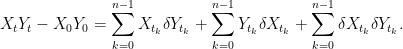
The gamblers winnings can be defined by a stochastic process  representing his net gain (or loss) just before the n’th toss. Let
  be a sequence of independent random variables with
  . Here,
  represents the outcome of the n’th toss, with 1 referring to a head and -1 referring to a tail. Set
  and
and
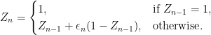
This is a martingale with respect to its natural filtration, starting at zero and, eventually, ending up equal to one. It can be converted into a local martingale by speeding up the time scale to fit infinitely many tosses into a unit time interval
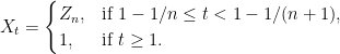
This is a martingale with respect to its natural filtration on the time interval  . Letting
  then the optional stopping theorem shows that
  is a uniformly bounded martingale on
  , continuous at
  , and constant on
  . This is therefore a martingale, showing that is a local martingale. However,
 ![{{\mathbb E}[X_1]=1\not={\mathbb E}[X_0]=0}](https://s0.wp.com/latex.php?latex=%7B%7B%5Cmathbb+E%7D%5BX_1%5D%3D1%5Cnot%3D%7B%5Cmathbb+E%7D%5BX_0%5D%3D0%7D&bg=ffffff&fg=000000&s=0&c=20201002) , so it is not a martingale. Continue reading “Local Martingales” →
, so it is not a martingale. Continue reading “Local Martingales” →


![{[0,t]}](https://s0.wp.com/latex.php?latex=%7B%5B0%2Ct%5D%7D&bg=ffffff&fg=000000&s=0&c=20201002)


 is a
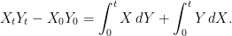
is a  can be interpreted as a
  represents the Lebesgue-Stieltjes integral of
  with respect to the
  to be
to be 
 . Then,
  and the stochastic integral
  agrees with the Lebesgue-Stieltjes integral, with probability one.
  is a sequence of predictable processes dominated by any such
  , so that
  for each
 of a function
  . This does, however, require restricting attention to differentiable functions. By integrating, it is possible to generalize to
  is such a function and
  is continuous, then the
  is well defined. The Lebesgue-Stieltjes integral further generalizes this to measurable integrands.
 is not defined using standard methods.
 such that the stopped processes
 for the processes locally in P. Choosing the sequence
  of stopping times shows that
  . A class of processes is said to be stable if
  is in P whenever X is, for all stopping times
  . For example, the
  is uniformly integrable. However, even if this is the case, it does not follow that the set of values of the process sampled at arbitrary stopping times is uniformly integrable.
![{X_\tau={\mathbb E}[X_t\mid\mathcal{F}_\tau]}](https://s0.wp.com/latex.php?latex=%7BX_%5Ctau%3D%7B%5Cmathbb+E%7D%5BX_t%5Cmid%5Cmathcal%7BF%7D_%5Ctau%5D%7D&bg=ffffff&fg=000000&s=0&c=20201002) for stopping times
for stopping times  . As sets of conditional expectations of a random variable are uniformly integrable, the following result holds.
 is uniformly integrable.
 is uniformly integrable.
 converges uniformly on compacts to a limit
 converges to the limit
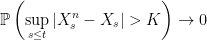
 .
.  . The absolute maximum process of a martingale is denoted by
  . For any real number
  , the
, the  -norm of a random variable
  is
is![\displaystyle \Vert Z\Vert_p\equiv{\mathbb E}[|Z|^p]^{1/p}.](https://s0.wp.com/latex.php?latex=%5Cdisplaystyle++%5CVert+Z%5CVert_p%5Cequiv%7B%5Cmathbb+E%7D%5B%7CZ%7C%5Ep%5D%5E%7B1%2Fp%7D.+&bg=ffffff&fg=000000&s=0&c=20201002)
 -norm of its terminal value, and bound the
  .
. . Then
  ,
,
![\displaystyle \lVert X^*_t\rVert_1\le\frac e{e-1}{\mathbb E}\left[\lvert X_t\rvert \log\lvert X_t\rvert+1\right].](https://s0.wp.com/latex.php?latex=%5Cdisplaystyle++%5ClVert+X%5E%2A_t%5CrVert_1%5Cle%5Cfrac+e%7Be-1%7D%7B%5Cmathbb+E%7D%5Cleft%5B%5Clvert+X_t%5Crvert+%5Clog%5Clvert+X_t%5Crvert%2B1%5Cright%5D.+&bg=ffffff&fg=000000&s=0&c=20201002)
 is bounded above by some finite value as
  runs through the positive reals.
 exists and is finite, with probability one.