The previous post introduced the notion of a stopping time  . A stochastic process
  can be sampled at such random times and, if the process is jointly measurable,
  will be a measurable random variable. It is usual to study adapted processes, where
  is measurable with respect to the sigma-algebra
  at that time. Then, it is natural to extend the notion of adapted processes to random times and ask the following. What is the sigma-algebra of observable events at the random time , and is measurable with respect to this? The idea is that if a set
  is observable at time then for any time
  , its restriction to the set
  should be in . As always, we work with respect to a filtered probability space
  . The sigma-algebra at the stopping time is then,
The restriction to sets in  is to take account of the possibility that the stopping time can be infinite, and it ensures that
  . From this definition, a random variable
  us
us  -measurable if and only if
  is -measurable for all times
  .
.
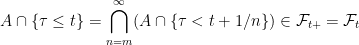
Similarly, we can ask what is the set of events observable strictly before the stopping time. For any time , then this sigma-algebra should include restricted to the event  . This suggests the following definition,
The notation  denotes the sigma-algebra generated by a collection of sets, and in this definition the collection of elements of
  are included in the sigma-algebra so that we are consistent with the convention
  used in these notes.
With these definitions, the question of whether or not a process is -measurable at a stopping time can be answered. There is one minor issue here though; stopping times can be infinite whereas stochastic processes in these notes are defined on the time index set  . We could just restrict to the set
  , but it is handy to allow the processes to take values at infinity. So, for the moment we consider a processes where the time index runs over
  , and say that is a predictable, optional or progressive process if it satisfies the respective property restricted to times in and
  is -measurable.
Lemma 1 Let be a stochastic process and be a stopping time.
- If is progressively measurable then is -measurable.
- If is predictable then is
 -measurable.
Proof: If is progressive then, as proven in the previous post, the stopped process  is also progressive and, hence, is adapted. It follows that
  is -measurable which, from the definition above, implies that
  is
is  -measurable.
Furthermore,  is -measurable and is zero when restricted to the set
  for all
  , so is also -measurable.
Now, consider a predictable process . Write  for the predictable sigma-algebra on
  . That is, the subsets of
  which are predictable when restricted to
  and such that
  is -measurable. Then, is -measurable. By the functional monotone class theorem, it is enough to prove the result for processes of the form
  for some pi-system of sets generating .
The predictable sigma algebra is generated by the sets  of the following forms,
-
![{S=(t,\infty]\times A}](https://s0.wp.com/latex.php?latex=%7BS%3D%28t%2C%5Cinfty%5D%5Ctimes+A%7D&bg=ffffff&fg=000000&s=0&c=20201002) for times and
for times and  . If
. If  then
then  which, by definition, is -measurable.
-
 for
for  . If then
  which is -measurable, and so is also -measurable.
⬜
So, the `adaptedness’ of measurable processes extends to stopping times. In fact, it is possible to go further and use this as an alternative definition of these sigma-algebras.
Lemma 2 Let be a random variable and be a stopping time. Then,
- is -measurable if and only if
 for some progressively measurable (or, optional) process .
- is -measurable if and only if
 for some predictable process .
Proof: If is -measurable, then the process  is adapted and right-continuous. Therefore, it is optional (and hence, progressive) and clearly .
For the second statement, consider the set  of random variables which can be expressed as for a predictable process . The functional monotone class theorem can be used to show that contains all -measurable random variables. First, is clearly closed under taking linear combinations. Second, if
  is increasing to the limit then there exists predictable processes
  with
with  . Then,
  is also in .
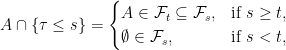
Finally, it just needs to be shown that  for all in a pi-system generating . By definition, the following sets generate .
-
 . In this case,
  with
with  .
.
-
 for and . Then, with
  .
.
In both these cases, is left-continuous and adapted and, hence, is predictable. ⬜
This result gives the main motivation for the definitions of and . For the remainder of this post, I state and prove several simple results which are useful for general applications of stopping times.
Lemma 3 Any stopping time is both and -measurable.
Proof: The deterministic process  is trivially adapted and both left and right-continuous, so it is predictable and optional. Consequently, by the previous lemma,
  is and -measurable. ⬜
Next, the sigma-algebras are increasing in the sense that we would hope.
Lemma 4 For any stopping time ,
If  is any other stopping time then,
If, furthermore,  whenever
  then
then  .
.
Proof: This proof makes use of Lemma 2. First, by the lemma, every -measurable set can be written in the form  for a predictable process . However, as predictable processes are progressive, will also be in .
Now suppose that is  (resp.
  ) measurable. Then, there is a progressive (resp. predictable) process satisfying
  . As the stopped process
  is also progressive (resp. predictable) it follows that
  is (resp. )-measurable.
Finally, suppose that whenever and that  . Then
is a left-continuous and adapted at finite times, and is -measurable. Hence, it is predictable process and is -measurable. ⬜
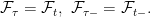
The sigma-algebras satisfy the expected left and right-limits. In the following lemma, the first statement says that right-continuity of a filtration extends to arbitrary stopping times. The second says that can indeed be interpreted as a left-limit. However, this statement does not say anything much for arbitrary stopping times, because it is not in general possible to strictly approximate them from the left in this way. If such a sequence  does indeed exist then the stopping time is called predictable.
Lemma 5 Let  be stopping times. Then
- If the filtration
 is right-continuous and
  for each
  then
then
- If
 , with a strict inequality whenever , then
Proof: Starting with the first statement, we know that  . So, it just needs to be shown that any
  is in . Any such set satisfies
Then, by right-continuity of the filtration, for any 
as required.
For the second statement, we know that  , so it is only necessary to prove that there is a generating set for lying in
  . As
. As  it is enough to consider sets of the form
  for . However
as required. ⬜
As should be the case, the definition of the sigma-algebras at a constant stopping time is consistent with the filtration.
Lemma 6 If  is equal to the constant value then,
Proof: If then for all times  ,
,
showing that  . Conversely, if then
  as required.
This shows that  . The equality
  follows by taking left limits and applying the previous lemma. ⬜
Given two stopping times  it follows from the definitions that
  and
and  . So,
. So,  is in and, by symmetry, is also in . Furthermore, these two sigma-algebras coincide when restricted to this set. For a sigma-algebra
  on
on  , and a subset
  , we use
  to denote the sigma-algebra on S consisting of sets
  for
for  .
.
Lemma 7 If are stopping times then
Proof: If  is measurable then
  is in and . The reverse inclusion follows by exchanging
  and .
and .
Next,  is generated by sets in
  , and by sets of the form
  for
for  which, restricted to , coincide with
  . So,
. So,  , and the reverse inclusion follows by exchanging and . ⬜
Given a stopping time taking values in a countable set of times, the following result is often useful to show that a set is in the sigma algebra by checking it at each of the fixed times.
Lemma 8 Let  be stopping times such that
  for all
  .
.
A set  is in if and only if
  for each .
Proof: By the previous lemma, if then  . Conversely,
as required. ⬜
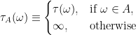
Finally, the following result is used to construct new stopping times out of old ones. If we wait until a time occurs, and then decide to either use that time or not based on an -measurable event, the result is again a stopping time.
Lemma 9 Let be a stopping time and . Then,
is also a stopping time.
Proof: This follows from the following
for all . ⬜


Dear Almost sure,

In lemma 7, do you want to show
Thanks
Yes! I’ll fix it. Thanks
Dear Georges, ?
?
Excuse me if I am wrong, but in the proof of Lemma 2, last but one line, shouldn’t it be
You’re right. I fixed it, thanks.
Thanks for your answer. Did you also by any chance see my question on the Stochastic Integral ?
Hello George,
I recently meet the problem on consistency of probability measures. Given a sequence of probability measures Q_n, how is it possible to check that they are consistent? The definition seems impractical. What I want is a method that we can actually apply facing concrete examples. Also, where shall I start if I want to find counter-examples?
Thank you very much!
Hi, I am struggling with the definition of the “stopping-time sigma-algebra” (aka sigma algebra at stopping time). You state that, “The idea is that if a set is observable at time
  then for any time
  , its restriction to the set
  should be in
  .” Is it possible to get a concrete example please? Thanks.
Hi, Thanks for the excellent posts. One question: Why is the sigma algebra at a stopping time “tau” not defined as the sigma algebra generated by tau, in the first place? How is this notion related to the (standard) definition that you have given above? I vaguely recall some mention (not sure in which reference) that the former definition is not operationally useful to perform the related analysis–is that so or are there other reasons?
Consider the case where is constant, equal to a deterministic time
  . Then
  . With the definition you suggest,
  would be trivial. More generally, the sigma algebra generated by
  would miss out lots of events observable at the stopping time. We want
  to be
to be  -measurable for any reasonably regular adapted process X.
I have been trying to prove if and
and  are stopping times and
  , then
  . Any suggestions on how to proceed?
You can try using . From the definitions of the two sigma-algebras, this is in
  . Take the union over a countable dense set for t. Alternatively use the fact that
  is left-continuous and adapted, so
  is
is  measurable.
Nitpicking: “resp.” in Lemma 2 is quite confusing. Probably you meant just “or”? [GL: Fixed, thanks!]
Why is the “progressive” condition used to show that $X_\tau$ is $\mathcal F_\tau$-measurable? Is adapted $X$ not enough?
Dear George,
I believe there is a mistake in the last part of the proof of Lemma 4. The suggested process X is not left-continuous. Take s<= \sigma < t then X_t-X_s=0 while if \sigma<s<t then X_t-X_s=1. I also believe that in the second bullet point in the proof of Lemma 2, the inequality between s and t is in the wrong direction.
Nevermind the first comment, that is obviously left-continuity. I stand by the second comment nonetheless
1
1ph5ATRgh
1*1
1-1; waitfor delay ‘0:0:15’ —
1-1); waitfor delay ‘0:0:15’ —
1′”
@@KG07j
1*696*691*0
1+701-696-5
1*535*530*0
1+540-535-5
1*796*791*0
1+801-796-5
1*475*470*0
1+480-475-5
1*308*303*0
1+313-308-5
1*786*781*0
1+791-786-5
1*761*756*0
1+766-761-5
1*559*554*0
1+564-559-5