Quadratic Variations and Integration by Parts

George Lowther Stochastic Calculus Notes, Stochastic Integration 18 January 1025 February 22

A major difference between standard integral calculus and stochastic calculus is the existence of quadratic variations and covariations. Such terms show up, for example, in the stochastic version of the integration by parts formula.

For motivation, let us start by considering a standard argument for differentiable processes. The increment of a process ${X}$ over a time step ${\delta t>0}$ can be written as ${\delta X_t\equiv X_{t+\delta t}-X_t}$ . The following identity is easily verified,

$\displaystyle \delta XY = X\delta Y + Y\delta X + \delta X \delta Y.$

(1)

Now, divide the time interval ${[0,t]}$ into ${n}$ equal parts. That is, set ${t_k=kt/n}$ for ${k=0,1,\ldots,n}$ . Then, using ${\delta t=1/n}$ and summing equation (1) over these times,

$\displaystyle X_tY_t -X_0Y_0=\sum_{k=0}^{n-1} X_{t_k}\delta Y_{t_k} +\sum_{k=0}^{n-1}Y_{t_k}\delta X_{t_k}+\sum_{k=0}^{n-1}\delta X_{t_k}\delta Y_{t_k}.$

(2)

If the processes are continuously differentiable, then the final term on the right hand side is a sum of ${n}$ terms, each of order ${1/n^2}$ , and therefore is of order ${1/n}$ . This vanishes in the limit ${n\rightarrow\infty}$ , leading to the integration by parts formula

$\displaystyle X_tY_t-X_0Y_0 = \int_0^t X\,dY + \int_0^t Y\,dX.$

Now, suppose that ${X,Y}$ are standard Brownian motions. Then, ${\delta X,\delta Y}$ are normal random variables with standard deviation ${\sqrt{\delta t}}$ . It follows that the final term on the right hand side of (2) is a sum of ${n}$ terms each of which is, on average, of order ${1/n}$ . So, even in the limit as ${n}$ goes to infinity, it does not vanish. Consequently, in stochastic calculus, the integration by parts formula requires an additional term, which is called the quadratic covariation (or, just covariation) of ${X}$ and ${Y}$ .

There are several methods of defining quadratic variations, but my preferred approach is to use limits along partitions. A stochastic partition ${P}$ of the nonnegative real numbers ${{\mathbb R}_+}$ is taken to mean a sequence of stopping times, starting at zero and increasing to infinity in the limit,

$\displaystyle P = \left\{0=\tau_0\le\tau_1\le\tau_2\le\cdots\uparrow\infty\right\}.$

(3)

Along such a partition, the approximation ${[X]^P}$ to the quadratic variation of ${X}$ and the approximation ${[X,Y]^P}$ to the covariation of ${X}$ and ${Y}$ is,

$\displaystyle \setlength\arraycolsep{2pt} \begin{array}{rl} \displaystyle [X]^P_t &\displaystyle= \sum_{n=1}^\infty\left(X_{\tau_n\wedge t}-X_{\tau_{n-1}\wedge t}\right)^2,\smallskip\\ \displaystyle [X,Y]^P_t &\displaystyle = \sum_{n=1}^\infty\left(X_{\tau_n\wedge t}-X_{\tau_{n-1}\wedge t}\right)\left(Y_{\tau_n\wedge t}-Y_{\tau_{n-1}\wedge t}\right). \end{array}$

(4)

Note that the times ${\tau_n\wedge t}$ are eventually constant and equal to ${t}$ , so the sums above only contain finitely many nonzero terms. If ${P}$ is a stochastic partition of ${{\mathbb R}_+}$ then ${P^t\equiv\{\tau_0\wedge t,\tau_1\wedge t,\ldots\}}$ is a partition of the interval ${[0,t]}$ . Its mesh is the longest subinterval

$\displaystyle \vert P^t\vert = \max_n\left(\tau_n\wedge t-\tau_{n-1}\wedge t\right).$

For stochastic partitions, this is a random variable. The quadratic variation and covariation are then equal to the limit of the approximations (4) as the mesh goes to zero. At any fixed time, this limit converges in probability. However, looking at the paths of the processes, the stronger property of uniform convergence on compacts in probability (ucp) is obtained. The proof is given further below.

Theorem 1 (Quadratic Variations and Covariations) Let ${X,Y}$ be semimartingales. Then, there exist cadlag adapted processes ${[X]}$ and ${[X,Y]}$ satisfying the following.

For any sequence ${P_n}$ of stochastic partitions of ${{\mathbb R}_+}$ such that, for each ${t\ge 0}$ , the mesh ${\vert P_n^t\vert}$ tends to zero in probability as ${n\rightarrow\infty}$ , the following limits hold

$\displaystyle \setlength\arraycolsep{2pt} \begin{array}{rl} \displaystyle [X]^{P_n}&\displaystyle\xrightarrow{\rm ucp}[X],\smallskip\\ \displaystyle [X,Y]^{P_n}&\displaystyle\xrightarrow{\rm ucp}[X,Y], \end{array}$ (5)

as ${n\rightarrow\infty}$ . Furthermore, convergence also holds in the semimartingale topology.

The process ${[X]}$ is called the quadratic variation of ${X}$ and ${[X,Y]}$ is the (quadratic) covariation of ${X}$ and ${Y}$ . Note that, as ${[X,Y]^P}$ is symmetric and bilinear in ${X,Y}$ with ${[X,X]^P=[X]^P}$ , then the same holds for ${[X,Y]}$ . That is,

$\displaystyle \setlength\arraycolsep{2pt} \begin{array}{rl} &\displaystyle \left[ \lambda X+\mu Y,Z\right ] = \lambda [X,Z] + \mu [Y,Z],\smallskip\\ &\displaystyle \left[ X, \lambda Y+\mu Z\right ] = \lambda [X,Y] + \mu [X,Z],\smallskip\\ &\displaystyle [X,Y] = [Y,X],\ [X] = [X,X], \end{array}$

for semimartingales ${X,Y,Z}$ and real numbers ${\lambda,\mu}$ . It is clear that ${[X]_0=[X,Y]_0=0}$ . The following properties also follow easily from the definition. Recall that an FV process is a cadlag adapted process with almost surely finite variation over all bounded time intervals, and such processes are semimartingales.

Lemma 2

If ${X}$ is a semimartingale then ${[X]}$ is a cadlag adapted and increasing processes.

If ${X,Y}$ are semimartingales then ${[X,Y]}$ is an FV process.

Proof: Choose times ${s<t}$ . If ${P}$ is any stochastic partition as in (3) with ${\tau_m=s}$ for some ${m}$ then,

$\displaystyle [X]^P_t-[X]^P_s = \sum_{n=m+1}^\infty\left(X_{\tau_n\wedge t}-X_{\tau_{n-1}\wedge t}\right)^2\ge 0.$

Taking limits of such partitions gives ${[X]_t-[X]_s\ge 0}$ as required. Then, the polarization identity expresses ${[X,Y]=([X+Y]-[X-Y])/4}$ as the difference of increasing processes and, as such, is an FV process. ⬜

In particular, quadratic variations variations and covariations are semimartingales. The following differential notation is sometimes used,

$\displaystyle \setlength\arraycolsep{2pt} \begin{array}{rl} \displaystyle dX^2 &\displaystyle\equiv d[X],\smallskip\\ \displaystyle dXdY &\displaystyle\equiv d[X,Y]. \end{array}$

The stochastic version of the integration by parts formula is as follows. Sometimes, this result is used as the definition of quadratic covariations instead of using partitions as above.

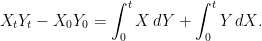
Theorem 3 (Integration by Parts) If ${X,Y}$ are semimartingales then

$\displaystyle XY = X_0Y_0+\int X_{-}\,dY + \int Y_{-}\,dX+[X,Y].$ (6)

The proof of this is given along with the existence of quadratic variations below. The special case with ${X=Y}$ is often useful,

$\displaystyle X^2 = X_0^2 + 2\int X_{-}\,dX + [X].$

(7)

Note that, in differential notation (6) is simply

$\displaystyle dXY = X_{-}dY + Y_{-}dX + dXdY,$

which is the stochastic differential version of equation (1). As ${[X,Y]}$ is a semimartingale, the following corollary of the integration by parts formula is obtained.

Corollary 4 If ${X,Y}$ are semimartingales, then so is ${XY}$ .

Quadratic Variation of Brownian motion

As standard Brownian motion, ${B}$ , is a semimartingale, Theorem 1 guarantees the existence of the quadratic variation. To calculate ${[B]_t}$ , any sequence of partitions whose mesh goes to zero can be used. For each ${n}$ , the quadratic variation on a partition of ${n}$ equally spaced subintervals of ${[0,t]}$ is

$\displaystyle V^n\equiv \sum_{k=1}^n (B_{kt/n}-B_{(k-1)t/n})^2.$

The terms ${B_{kt/n}-B_{(k-1)t/n}}$ are normal with zero mean and variance ${t/n}$ . So, their squares have mean ${t/n}$ and variance ${2t^2/n^2}$ , giving the following for ${V^n}$ ,

$\displaystyle \setlength\arraycolsep{2pt} \begin{array}{rl} \displaystyle {\mathbb E}[V^n] &\displaystyle = \sum_{k=1}^n{\mathbb E}\left[(B_{kt/n}-B_{(k-1)t/n})^2\right]=\sum_{k=1}^nt/n=t,\smallskip\\ \displaystyle {\rm Var}[V^n] &\displaystyle = \sum_{k=1}^n {\rm Var}\left[(B_{kt/n}-B_{(k-1)t/n})^2\right]=\sum_{k=1}^n2t^2/n^2=2t^2/n. \end{array}$

The variance vanishes as ${n}$ goes to infinity, ${{\mathbb E}[(V^n-t)^2]\rightarrow 0}$ . This gives the quadratic variation as simply

$\displaystyle [B]_t = t.$

(8)

Using bilinearity of quadratic covariations, this result can be generalized to obtain the quadratic covariations of correlated Brownian motions. Two Brownian motions ${B^1,B^2}$ have correlation ${\rho}$ if, for each ${t>s}$ , ${\delta B^1\equiv B^1_t-B^1_s}$ and ${\delta B^2\equiv B^2_t-B^2_s}$ are independent of ${\mathcal{F}_s}$ and jointly normal with correlation ${\rho}$ . That is, their covariance is ${\rho(t-s)}$ . If ${X=\lambda(B^1 + B^2)}$ for a constant ${\lambda}$ then it follows that ${\delta X\equiv X_t-X_s}$ is normal with variance

$\displaystyle {\mathbb E}[(\delta X)^2]=\lambda^2{\mathbb E}[(\delta B^1)^2+(\delta B^2)^2+2\delta B^1\delta B^2]=\lambda^2(2+2\rho)(t-s).$

If we choose ${\lambda^2=1/(2+2\rho)}$ then this shows that ${X}$ is a standard Brownian motion, with quadratic variation given by (8). Bilinearity of covariations can be applied,

$\displaystyle t=[X]_t=\lambda^2([B^1]_t+2[B^2]_t+2[B^1,B^2]_t)=2\lambda^2(t+[B^1,B^2]_t).$

Substituting back in ${\lambda^2=1/(2+2\rho)}$ , rearranging this expression gives the following for the covariation of the correlated Brownian motions,

$\displaystyle [B^1,B^2]_t=\rho t.$

In particular, independent Brownian motions have zero covariation.

Existence of Quadratic Variations

It remains to prove that the quadratic variations and covariations defined by Theorem 1 do indeed exist, and then that the integration by parts formula is satisfied. In fact, it is easier to first define ${[X,Y]}$ to be the unique process satisfying equation (6), and then show that the limit stated by Theorem 1 holds. It follows directly from this definition that ${[X,Y]}$ is a cadlag adapted process. Taking ${[X]\equiv [X,X]}$ then it is enough to prove the limit ${[X]^{P_n}\rightarrow [X]}$ . The corresponding limit for the covariation will follow from the polarization identities ${4[X,Y]^P=[X+Y]^P-[X-Y]^P}$ and ${4[X,Y]=[X+Y]-[X-Y]}$ .

The method of proof will be to express ${[X]^P-[X]}$ as a stochastic integral, so that the dominated convergence theorem can be used to show that this tends to zero as the mesh of the partition vanishes. Fixing a time ${t}$ and partition ${P}$ , as in equation (3), the square of the change in ${X}$ across an interval, ${\delta X_n\equiv X_{\tau_n\wedge t}-X_{\tau_{n-1}\wedge t}}$ , can be rearranged as

$\displaystyle \delta X_n^2 = X_{\tau_n\wedge t}^2-X_{\tau_{n-1}\wedge t}^2-2X_{\tau_{n-1}\wedge t}\delta X_n.$

The last term on the right can be expressed as the integral of ${2X_{\tau_{n-1}}}$ with respect to ${X_s}$ between the limits ${\tau_{n-1}\wedge t}$ and ${\tau_n\wedge t}$ . Also substituting in the integration by parts formula (7) for the first two terms,

$\displaystyle \delta X_n^2 = [X]_{\tau_n\wedge t}-[X]_{\tau_{n-1}\wedge t}+2\int_0^t (X_{s-}-X_{\tau_{n-1}})1_{\{\tau_{n-1}<s\le \tau_n\}}\,dX_s.$

If we sum this expression over ${n}$ , then the integrand in the final term becomes

$\displaystyle \alpha^P_s\equiv\sum_{n=1}^\infty (X_{s-}-X_{\tau_{n-1}})1_{\{\tau_{n-1}< s\le \tau_n\}}$

giving the following expression for the quadratic variation along a partition

$\displaystyle [X]^P_t = [X]_t + 2\int_0^t \alpha^P \,dX.$

(9)

Now, let ${P_k}$ be a sequence of such partitions whose mesh ${\vert P^t_k\vert}$ goes to zero as ${k\rightarrow\infty}$ . It is clear from the left continuity of ${X_{s-}}$ that ${\alpha^{P_k}_s\rightarrow 0}$ . Furthermore, ${\vert \alpha^{P_k}_s\vert\le 2\sup_{u < s}\vert X_u\vert}$ , which is locally bounded. Then, the dominated convergence theorem says that ${\int\alpha^{P_k}\,dX\rightarrow 0}$ , converging ucp and in the semimartingale topology. Putting this into (9) gives ${[X]^{P_k}\rightarrow [X]}$ as required.

This proves the result in the case where ${\vert P^t_k\vert\rightarrow 0}$ everywhere for all ${t}$ . The final thing to do is to generalize to the case where ${\vert P^t_k\vert}$ only goes to zero in probability. However, in that case it is possible to pass to a subsequence ${\tilde P_k}$ satisfying ${{\mathbb P}(\vert\tilde P_k^{t}\vert>1/k)<2^{-k}}$ for all ${t\le k}$ . The Borel-Cantelli lemma guarantees that ${\vert \tilde P_k^t\vert\rightarrow 0}$ almost everywhere for all ${t}$ . The above proof then shows that ${[X]^{\tilde P_k}\rightarrow [X]}$ , converging ucp and in the semimartingale topology. Then, by this same argument, every subsequence of ${[X]^{P_k}}$ itself has a subsequence converging to ${[X]}$ . As the cadlag processes under the ucp and semimartingale topologies is a metric space, this is enough to guarantee convergence of the original sequence.

Published by George Lowther

View all posts by George Lowther

Published 18 January 1025 February 22

46 thoughts on “Quadratic Variations and Integration by Parts”

Alekk says:

3 June 10 at 12:24 PM

Dear George,

do the partitions need to be nested in order to define the quadratic variation. I still remember having done one exercise in Peres’ book on Brownian motion that showed that some weird stuffs can happen for non-nested partitions. On the other hand, it seems like you do not need this assumption here, and I remember that the first time I learned my stochastic analysis it was not needed as well. I guess I am missing something, somewhere …

Many thanks,
Alekk

Reply
1. George Lowther says:
  
  3 June 10 at 12:46 PM
  
  No, the partitions do not need to be nested.
  
  You can show that, if they are nested and fixed times are used ( rather than stopping times) then, for Brownian motion, you get almost sure convergence to the quadratic variation. This follows from martingale convergence. That probably what the exercise was referring to.
  
  The weaker notion of convergence in probability is used in my post. This works for all semimartingales and does not need nested partitions.
  
  Reply
Alekk says:

3 June 10 at 3:16 PM

It is something a little bit more annoying: it can be shown (see in Peres’s book, http://www.stat.berkeley.edu/~peres/) that they exist (necessarily non-nested) sequences of deterministic partitions $P_N$ such that almost surely, $\limsup [B]^{P_N}_t = +\infty$ . Indeed, this is not a contradiction with the convergence in probability, but I just find it quite deranging.

I just read again this passage of Peres’ book (exercice 1.13): there even exist random sequences of partitions $P_N$ such that $\lim [B]^{P_N}_t = +\infty$ : this time this is even more annoying, isnt it ? (I have not done myself this exercice with random partitions, though)

Reply
1. George Lowther says:
  
  4 June 10 at 1:14 AM
  
  Well, whether you find that annoying depends on your point of view, but I don’t think it should be too surprising. Convergence in probability does not usually tell you much about convergence at individual points of the probability space.
  E.g., take any sequence of IID random variables with unbounded support (normal, say). Even though it will be bounded in probability, their limsup will be infinite. Then, multiplying them by a sequence of real numbers converging to zero slowly enough gives a sequence of rvs tending to zero in probability but whose limsup is infinite, and there will be a (random) subsequence which goes to infinity.
  
  Also, given a sample path of BM, with probability one there will be a sequence of nested partitions along which its QV is infinite. There will also be nested partitions along which its QV is zero (as for any continuous function) and any number in between. So, you can construct nested random partitions partitions along which the QV is any nonnegative number you like.
  
  Similar things happen for other situations where you have convergence in probability. E.g., there are sequences of predictable integrands $\alpha_n$ converging uniformly to zero such that $\limsup_n\int_0^1\alpha_n\,dB=\infty$ . The dominated convergence theorem gives convergence in probability, but not almost sure convergence (although almost sure convergence does occur for monotone sequences of integrands).
  
  If a sequence converges in probability quickly enough, then Borel-Cantelli gives almost sure convergence. Otherwise you need something special, such as martingale convergence.
  
  Reply
Alekk says:

4 June 10 at 2:18 AM

thank you very much for these explanations!

I always thought of the concept of quadratic variation as something very stable and robust, and this is why I was a little bit annoyed about these kind of pathologies. Also, from a practical point of view, this might be a little bit annoying: if we observe an unknown stochastic process, a diffusion say, and want to do some kind of inference on the volatility function, we might want to have good properties for the quadratic variation function. In general, I think that this is a difficult (and important) statistical problem.

Reply
NK says:

24 November 10 at 2:35 AM

Dear George,

I was wondering how to interpret $\int_0^t 2 X_{s-} dX_s$ , $X_0=0$ . The explicit solution when $X_s$ is geometric Brownian motion or a jump-diffusion (Levy process), is $(E(X_t))^2$ . But I do not have an intuitive understanding of why this is so (and, therefore, why it isn’t for alternative processes).

Thanks!,

Nikunj

Reply
1. George Lowther says:
  
  7 December 10 at 12:15 AM
  
  Hi,
  
  I’m not sure quite what you are asking. The explicit solution is $X_t^2-[X]_t$ . That’s stochastic, and not the same thing as $(E(X_t))^2$ .
  Maybe I can help if you clarify your question? (and apologies for being slow to respond.)
  
  Reply
NK says:

7 December 10 at 4:45 AM

My bad; I forgot to add in the expectation. I meant $E \int_0^t 2 X_s dX_s = \left ( \mbox{E} X_t \right )^2$ . So, for example, suppose $X_s = \ln P_s/P_0$ where $d \ln P_s = (\mu - \frac{1}{2} \sigma^2 ) ds + \sigma dW$ with $P_0 = 1$ . Then, $\mbox{E} \int_0^t 2 X_s dX_s = \int_0^t 2 (\mu - \frac{1}{2} \sigma^2)^2 ds = \left ( (\mu - \frac{1}{2} \sigma^2) t \right )^2 = \left ( \mbox{E} \ln P_t/P_0 \right )^2 = (\mbox{E} (X_t))^2$ .

Reply
1. George Lowther says:
  
  8 December 10 at 12:29 AM
  
  ah, ok. That is equivalent to $\mathbb{E}\left[ [X]_t\right] = {\rm Var}(X_t)$ . This holds for any square integrable martingale (it’s just the Ito Isometry). It also holds for any process of the form $X_t= M_t+b_t$ where M is a square integrable martingale and $b_t$ is a deterministic FV process (which does not affect either the variance or quadratic variation). This includes Brownian motion plus drift and square integrable Lévy processes. It’s a consequence of ‘orthogonality’ of increments, so that
  
  $\displaystyle{\rm Var}\left(X_t-X_0\right)=\sum_{k=1}^n{\rm Var}\left(X_{t_k}-X_{t_{k-1}}\right)$
  
  for times $0=t_0\le t_1\le\cdots\le t_n=t$ . Letting the mesh $\max_k\vert t_k-t_{k-1}\vert$ go to zero (and assuming nice integrability properties), the right hand side will converge to $\mathbb{E}\left[ [X]_t\right]$ .
  Processes where the drift term $b_t$ is stochastic will not satisfy this. E.g., $X_t=\int_0^t W_s\,ds$ has zero quadratic variation, but nonzero variance.
  
  Reply
  1. NK says:
    
    14 December 10 at 10:33 PM
    
    Thank you very much! This is really helpful!
    
    Reply
HanaPipers says:

7 February 12 at 11:33 PM

🙂

Reply
J says:

25 May 12 at 9:02 PM

I have a question on something that has really been troubling me about quadratic variations…if you could help, it would really be awesome..

It says on http://planetmath.org/encyclopedia/QuadraticVariation.html that ” it can be shown if any continuous deterministic process has a well defined quadratic variation along all partitions, then it is zero.” A brownian motion almost surely has quadratic variation t. However, suppose we generate a Brownian motion path and take it as fixed. Now, it is a deterministic path and should have zero quadratic variation??

More specifically, suppose we have the process d X_t = X_t d B_t + X_t d Z_t, where B_t and Z_t are independent Brownian motions. Suppose we condition X_t in [0,T] on a particular path B_{[0,T]}. So the path of B_t is now deterministic. Then, would we still use Ito for d f(X_t) (which follows from quadratic variation)??

would d f(X_t) = f_x(X_t) dX_t + .5 X_t^2 f_xx(X_t) dt or d f(X_t) = f_x(X_t) dX_t + X_t^2 f_xx(X_t) dt ??

My intuition tells me it should be the former since why would we apply Ito to a (now) deterministic process B_t ?

Thank you very much in advance for your insight into this..

Reply
1. George Lowther says:
  
  26 May 12 at 2:59 AM
  
  Actually, individual sample paths of Brownian motion do not have well defined quadratic variation. At least, not if you define the quadratic variation along arbitrary partitions. You can (almost-surely) find a sequence partitions with mesh going to zero on which the quadratic variation tends to zero, and other partitions on which the quadratic variation tends to infinity. See, also, the discussion with Alekk above.
  
  Reply
J says:

26 May 12 at 4:46 AM

thank you. that’s quite interesting.

For applications this seems quite strange. one often poses a model and we then try to fit it to past data. the model may include a brownian motion (or similar path) which we assume we have observed completely from past data. (for instance, in the simple example I’ve given above, suppose B_t is observed and we wish to find the conditional distribution of the function f(X_t) given its observed path.)

If the quadratic variation is not well-defined for any sample path (and we assume the historical data comes from such a sample path), how can we even approach such a problem?

thank you again for any insight!

Reply
1. George Lowther says:
  
  26 May 12 at 12:23 PM
  
  The quadratic variation can be defined on each sample path if you use a fixed sequence of partitions, independently of the values on the particular path. Although, it still might not converge on individual paths if the mesh doesnt go to zero fast enough. Practically, that doesn’t matter. Pick your partition, sample the process at those times and calculate the quadratic variation with the necessary error bounds. It is only if you were going to choose the partition in a way depending on the values that the process samples take that it would be possible to go wrong.
  
  Reply
J says:

3 June 12 at 9:18 PM

Thank you. Your answers have been very helpful as I try to understand this.

So, are you saying, even if I choose a deterministic partition a priori, it is not guaranteed that the quadratic variation for a single path of a Brownian motion will converge as i refine my mesh?

Also, since B_t is a realization of a single path, the integral f(X_t) = […..] + f'(X_t) d B_t is not well-defined (where X_t = Z_t + B_t and I observe B_t, as earlier). It is not well-defined in the mean square sense and obviously not the lebesgue-stieljes sense (even if the function f has nice properties, I believe). I realize there has been some theoretical work on pathwise construction of such integrals. However, more importantly, how do we know a standard euler method converges to the correct integral?

These questions seems to be brushed under the rug in the literature since; for instance, the Zakai equation also integrates against a single observed path of a Brownian motion, but I see no mention of this technical issue in the literature (they appear to just use Euler).

Reply
1. George Lowther says:
  
  6 June 12 at 2:21 AM
  
  Hi. Sorry about being a bit slow to respond. Its a bit late to be writing a long response right now, but I’ll just mention that convergence of the (approximations to) the integral is no problem, as long as your partitions use deterministic times or stopping times, and you are happy with convergence in probability. For Euler schemes, convergence in probability is what you probably want (or maybe L² convergence or similar for technical reasons). On individual paths, you are not guaranteed convergence if your sequence of partitions does not go to zero fast enough. However, any single fine enough partition will give you a tight confidence interval for the integral, if you want to do it in a precise way.
  
  Reply
Dhruv says:

12 November 12 at 5:44 AM

If we are to get d where X Y and Z are continuous semimartingales, what would that evaluate to? Also, how would one go about proving Doob’s L2 inequality?

Reply
Anonymous says:

16 November 16 at 2:44 AM

Hi George,

I have been reading your blog for a while as it has been a great source for me to understand stochastic calculus. I have the following question regarding quadratic covariation:

Let $(B_t^i,\mathcal F_t^i)$ , $i=1,2$ be two Brownian motions. Suppose the filtration $\{\mathcal F_t^1\}$ is contained in the filtration $\{\mathcal F_t^2\}$ . As a result, $B^2$ may not be adapted to $\{\mathcal F_t^1\}$ , while $B^1$ may not be a semi-martingale with respect to $\{\mathcal F_t^2\}$ .

1. Is there a way to define (or make sense of ) the quadratic covariation process $[B^1,B^2]$ ?
2. Given a sequence of refining partitions $\{\pi_n\}$ with $|\pi_n| \to 0$ , does the Riemann sum $\Sigma_{t_i \in \pi_n,t_i\leq t} (B_{t_{i+1}}^1-B_{t_i}^1)(B_{t_{i+1}}^2-B_{t_i}^2)$ converge in an sense?(say in probability,etc)

I have looked up things like Young integral and Follmer’s pathwise integral and none of those seem to be applicable in this case. Any help and suggestion would be greatly appreciated!

Reply
1. George Lowther says:
  
  17 November 16 at 12:00 AM
  
  Hi.
  
  You can always define the quadratic covariation using a sequence of partitions. It is not guaranteed to exist – I think I could come up with counterexamples for which it fails to converge in your situation.
  
  Reply
  1. Anonymous says:
    
    17 November 16 at 4:13 PM
    
    Hi George,
    
    Thank you for your reply. It’s not clear to me how a counterexample can be constructed. In most cases, the limit fails to exist due to its blowing up to infinity. In my case, the sequence of Riemann sums are already bounded in L2. If you have any idea on disproving convergence, please kindly let me know!
    
    best,
    Ryan
    
    Reply
    1. George Lowther says:
      
      18 November 16 at 8:38 AM
      
      Hi.
      
      I don’t have time to post a detailed construction right now, but there do exist examples where the correlation is -1 on some timescales and +1 on others. Computed along a sequence of partitions, the covariation will oscillate between +t and -t.
  2. Anonymous says:
    
    18 November 16 at 6:30 PM
    
    I agree that one can construct two Brownian motions such that, almost surely, the approximating sums converge to different limits along different sequence of partitions (I tried the Levy Ciesielski construction which seemed to work out nicely). However, the natural filtrations of those two Brownian motions does not necessarily satisfy the condition that one must be contained in the other, and I am not sure how to get away with this issue. Could you point me to some reference on the construction you mentioned? Thank you so much!
    
    Reply
    1. George Lowther says:
      
      18 November 16 at 7:29 PM
      
      I did think of a construction satisfying your properties, in response to your question. I should get time to post it later this weekend.
  3. Anonymous says:
    
    20 November 16 at 5:15 PM
    
    That’s great! I’m looking forward to seeing your construction!
    
    Reply
    1. George Lowther says:
      
      21 November 16 at 10:04 AM
      
      Hey. Apologies that I have not had chance yet to post the construction. It is a bit tricky, and I wasn’t 100% sure about it at first. I have given it a bit more thought though, and I think my construction works fine. I’ll try and post it later tonight.
  4. Anonymous says:
    
    22 November 16 at 3:12 PM
    
    No hurry! I’m also working on something similar. Please let me know once you have your construction posted.
    
    Reply
  5. Anonymous says:
    
    29 November 16 at 1:51 AM
    
    Hi Geroge,
    
    Sorry to bother you again. I am just wondering if you have made use of any sort of ergodic theory or theory of stationary sequence in your construction. I have tried many things and none of them worked, so I am hoping you can provide me some idea and insight into your construction. Thanks in advance!
    
    Ryan
    
    Reply
    1. George Lowther says:
      
      29 November 16 at 2:20 AM
      
      Sorry, haven’t had much time to write it out. But, the idea is to use Brownian bridge constructions on smaller and smaller timescales for which the correlations between the processes alternates between 1 and -1. Essentially, given an initial choice for $B^1$ , use a small rescaling of time such that on some fine enough partition, $B^1_{t_k}$ is $\mathcal{F}^2_{t_{k-1}}$ -measurable. Then interpolate between these times by linear interpolation plus a Browian bridge with correlation 1 or -1 with $B^2$ . This is a bit tricky, but I think it all works out and, taking the limit of such constructions gives a Brownian motion with correlation alternating between 1 and -1 in different timescales.
  6. Anonymous says:
    
    29 November 16 at 4:25 PM
    
    Thanks for your reply! I am assuming that you fix $B^2$ and $\mathbb(F)^2$ and construct $B^1$ . It seems to be crucial to require $B_{t_k}^1$ to be measurable with respect to $\mathcal(F)_{t_{k-1}}^2$ at each step to make sure the interpolation term is adpated. However, when you add in the Brownian bridge term, it seems that the property of $B^1$ being measurable one mesh size ahead w.r.t. $\mathcal(F)^2$ is destroyed. Is my understanding correct or am I missing something?
    
    Ryan
    
    Reply
    1. George Lowther says:
      
      29 November 16 at 4:50 PM
      
      You are correct, which is the point of the rescaling of time. i.e., before doing the Brownian Bridge interpolation, replace $B^1_t$ by $\alpha B^1_{\alpha^{-2}t}$ for $\alpha$ slightly greater than one.
  7. Ryan says:
    
    29 November 16 at 7:27 PM
    
    Hi George,
    
    I think i understand most of your idea of construction, but still cannot get it correctly. I guess I will wait and see if you have time to post it. Thank you very much for your help!
    
    Reply
  8. Ryan says:
    
    1 December 16 at 2:32 AM
    
    Dear George,
    
    Very sorry to bother you again as I still have some questions…
    1.My understanding of the Brownian bridge construction is that at every step of the construction, the approximating process, when evaluated at the mesh points, has the same joint distribution as a Brownian motion. This seems to fail after the time rescaling. Based on my understanding, to go from step n to n+1, you first replace $B_t^{1,n}$ by $\alpha B_{t/\alpha^2}^{1,n}$, then set $B_t^{1,n+1}=\frac{t-t_k^n}{t_{k+1}^n-t_k^n}B_{t_{k+1}^n}^{1,n}+\frac{t_{k+1}^n-t}{t_{k+1}^n-t_k^n}B_{t_k^n}^{1,n}+(-1)^n (t_{k+1}^n-t)\int_{t_k^n}^t \frac{\,dB_u^2}{t_{k+1}^n-u}$ for t \in [t_k^n,t_{k+1}^n]$. A time-rescaling seems to change the joint distribution of such process.
    2. I guess you have to start the construction somewhere away from time 0? Since rescaling of time by $\alpha$ close to 1 will not give you the desired “one mesh size ahead” measurability” at the first few mesh point.
    3. As you apply time-rescaling at each step of the construction, it’s not obvious if one can write down a formula describing the relation between the limiting process and the approximating process when evaluated at corresponding partition points.(as oppose to the standard case where the values are fixed from step to step) I am therefore wondering how do you compute covariation along different timescales and show they go to different limit.
    
    Again very sorry to bother you as this problem has puzzled me for quite a while and i really want to have a definite answer of it.
    Thanks!
    
    Reply
    1. George Lowther says:
      
      9 December 16 at 3:07 AM
      
      Hey, sorry, I really have not had much time to respond here. I do intend to answer this though.
      
      – Start by fixing the Brownian motion $B^2$ on a (fixed) filtered probability space $(\Omega,\mathcal{F},\{\mathcal{F}^2_t\}_{t\in[0,1]},\mathbb{P})$ . I will drop the superscript 2 just to make it easier to type. I’m also restricting the time index to [0,1] for simplicity.
      
      – We need to construct a process W, which is a Brownian motion under its natural filtration, and is adapted (but not a BM) w.r.t. the filtration $\mathcal{F}_t$ .
      
      If $\pi$ is a partition of [0,1], write $[B,W]^\pi$ for the covariation computed along $\pi$ . For the required counterexample, we want a sequence of partitions with mesh going to zero but where $[B,W]^\pi$ does not converge in probability.
      To do this, it is enough to have a method of constructing sequences of Brownian motions $W^n$ , adapted to the filtration, such that, for each n, $W^{n+1}$ can be chosen as close as we like to $W^n$ (ucp) and with $[B,W^{n+1}]_1=(-1)^n$ .
      
      If we can do this, then simultaneously choose partitions $\pi_n$ and $W^n$ as follows. Once $W^n$ is chosen,
      – choose $W^{n+1}$ close enough to $W^n$ to guarantee convergence of the sequence. e.g., $\mathbb{P}(\sup_t\lvert W^{n+1}_t-W^n_t\rvert > 2^{-n}) < 2^{-n}$
      – choose it close enough that $[B,W^{n+1}]^{\pi_k}$ is very close to $[B,W^{n}]^{\pi_k}$ for each $k\le n$ . For example, $\mathbb{P}(\sup_t\lvert [B,W^{n+1}]^{\pi_k}-[B,W^{n}]^{\pi_k}\rvert > 2^{-n}) < 2^{-n}$ .
      – choose the partition $\pi_{n+1}$ so that $[B,W^{n+1}]^{\pi_{n+1}}$ is very close to $(-1)^{n+1}$ . For example, $\mathbb{P}(\lvert[B,W^{n+1}]^{\pi_{n+1}}-(-1)^{n+1}\rvert > 2^{-n})< 2^{-n}. Then, it can be seen that$ latex W^n$ converges everywhere almost surely to a Brownian motion W. Furthermore, $(-1)^n[B,W]^{\pi_n}\to1$ , so $[B,W]^{\pi_n}$ does not converge.
    2. Ryan says:
      
      9 December 16 at 5:20 PM
      
      Dear George,
      
      Thanks for your reply! I am a little bit confused on where the Brownian bridge construction(time rescaling+brownian bridge interpolation) comes into play in your construction. I am also very curious on how to choose the partition. In my attempt the partition is fixed apriori to be the dyadic rationals.
      I have posted my question on MO:
      http://mathoverflow.net/questions/254788/brownian-motions-under-different-filtrations-quadratic-covariation-convergence
      You can share your solution there whenever you have some time. Thanks!
      
      Ryan
    3. George Lowther says:
      
      18 December 16 at 10:21 AM
      
      Hi. I’ve seen your mathoverflow post, and will get to it when I have some time. Unfortunately, I can’t at the moment, but will get back to it soon.
Ryan says:

23 May 17 at 12:35 AM

Dear George,

I am not sure if you remember, that six months ago, I consulted you this question on Brownian Motions under different filtrations and existence of quadratic covariation as limit of Riemann sum. You mentioned that you had a counter-example where the Riemann sum diverged.

This problem has remained a mystery to me until now. I have so far not been able to construct an counterexample, nor can I prove convergence. I am therefore wondering if you will have time to revisit this problem.

Thanks in advance!

Best,
Ryan

Reply
Jakob Ullmann says:

12 February 21 at 7:11 PM

Hi George,
first: thank you a lot for this blog, it’s an amazing source for stochastic calculus!
I am seriously confused about one point where your definition of the quadratic variation seems to be different from the one in Protter’s book. Apparently Protter defines the quadratic variation (and quadratic covariation) such that there is an additional term X_0 Y_0. Do you know what I mean? Otherwise I can provide more details… But there are a lot of instances there where it really makes a difference if one integrates over [0, t] or (0, t], for example… Is it possible that there are different conventions in the literature?

Reply
1. George Lowther says:
  
  12 February 21 at 11:54 PM
  
  Hi Jakob,
  
  Yes, this is just a matter of convention about what you do at time 0. Obviously any statement using one convention can be converted to an equivalent statement using the other. I’ll have to check for explicit definitions in the literature, but I am sure both are used. Similar issues occur in many places, such as the integral (as you mentioned), the definition of predictable processes and stopping times, the Doob-Meyer decomposition, dual projections, etc. In a way, you could consider extending your processes to negative times, by either being constant equal to their time 0 values, or equal to 0 there. I.e, do you consider your processes to have a jump at time zero or not? I made a choice (no jump at time 0) and stuck to it throughout these notes.
  
  Thanks
  George
  
  Reply
  1. George Lowther says:
    
    13 February 21 at 1:46 AM
    
    I checked a few sources. Rogers & Williams (Diffusions, Markov Processes, and Martingales), Metivier (Semimartingales), Jacod & Shiryaev (Limit Theorems for stochastic processes), Kallenberg (Foundations of Modern Probability) all have quadratic variation starting from 0. Protter is the outlier here, but either convention is fine IMO as long as you are consistent.
    
    Reply
Ilya Zakharevich says:

26 March 21 at 5:40 AM

In Theorem 3, the integrals make sense due to “consequence” to Lemma 5 in “Properties of…”. However, when one reads your notes non-linearly, this reduction is quite hard to find! It seems that a hyperlink would help a lot… Thanks!

Reply
stefanperko says:

24 September 21 at 11:05 AM

I was a bit confused about your derivation of (2). I think maybe you meant $t_k = tk/n$ ?

Reply
1. George Lowther says:
  
  25 February 22 at 1:42 PM
  
  I did mean that, thanks!
  Fixed.
  
  Reply
Julian says:

25 January 22 at 9:14 PM

I am not sure how you get the inequality $|\alpha^{P_k}| \le 2|X_{-}|$ in the final proof. For instance if you have $X_{-}(s)=0$ then $|\alpha^{P_k}(s)| = |X_{\tau_{n-1}}(s)|$ , which may not be zero. How do you explicitly get this inequality for all $k$ ?

Reply
1. George Lowther says:
  
  20 February 22 at 4:40 PM
  
  Well spotted! This was a typo really, I should have used the running maximum of X rather than X itself. I fixed it.
  
  Reply
Pingback: What’s the ∫T0(T−s)dWsint_0^T (T – s) dW_s? – Math Solution

	Anonymous on About
	Anonymous on About
	Anonymous on The Stochastic Integral
	Anonymous on Bessel Processes
	Anonymous on Bessel Processes
	Stat Prof on Pathwise Regularity of Optiona…
	Yang Chu on Spitzer’s Formula
	Anonymous on About
	Anonymous on Continuous Processes with Inde…
	Anonymous on Continuous Processes with Inde…

Quadratic Variation of Brownian motion

Existence of Quadratic Variations

Related

Published by George Lowther

46 thoughts on “Quadratic Variations and Integration by Parts”

Leave a reply to HanaPipers Cancel reply