Model-Independent Discrete Barrier Adjustments

I continue the investigation of discrete barrier approximations started in an earlier post. The idea is to find good approximations to a continuous barrier condition, while only sampling the process at a discrete set of times. The difference now is that I will look at model independent methods which do not explicitly depend on properties of the underlying process, such as the volatility. This will enable much more generic adjustments which can be applied more easily and more widely. I point out now, the techniques that I will describe here are original research and cannot currently be found in the literature outside of this blog, to the best of my knowledge.

Recall that the problem is to compute the expected value of a function of a stochastic process X,

$\displaystyle V={\mathbb E}\left[f(X_T);\;\sup{}_{t\le T}X_t \ge K\right]$

(1)

which depends on whether or not the process crosses a continuous barrier level K. In many applications, such as with Monte Carlo simulation, we typically only sample X at a discrete set of times 0 < t₁ < t₂ < ⋯< t_n = T. In that case, the continuous barrier is necessarily approximated by a discrete one

$\displaystyle V={\mathbb E}\left[f(X_T);\;\sup{}_{i=1,\ldots,n}X_{t_i}\ge K\right].$

(2)

As we saw, this converges slowly as the number n of sampling times increases, with the error between this and the limiting continuous barrier (1) only going to zero at rate 1/√n.

A barrier adjustment as described in the earlier post is able to improve this convergence rate. If X is a Brownian motion with constant drift μ and positive volatility σ, then the discrete barrier level K is shifted down by an amount βσ√δt where β ≈ 0.5826 is a constant and δt = T/n is the sampling width. We are assuming, for now, that the sampling times are equally spaced. As was seen, using the shifted barrier level in (2) improves the rate of convergence. Although we did not theoretically derive the new convergence rate, numerical experiment suggests that it is close to 1/n.

Another way to express this is to shift the values of X up,

$\displaystyle M_i=X_{t_i}+\beta\sigma\sqrt{\delta t}.$

(3)

Then, (2) is replaced to use these shifted values, which are a proxy for the maximum value of X across each of the intervals (t_i-1, t_i),

$\displaystyle V={\mathbb E}\left[f(X_T);\;\sup{}_{i=1,\ldots,n}M_i\ge K\right].$

(4)

As it is equivalent to shifting the level K down, we still obtain the improved rate of convergence.

This idea is especially useful because of its generality. For non-equally spaced sampling times, the adjustment (3) can still be applied. Now, we just set δt = t_i – t_i-1 to be the spacing for the specific time, so depends on index i. It can also be used for much more general expressions than (1). Any function of X which depends on whether or not it crosses a continuous barrier can potentially make use of the adjustment described. Even if X is an Ito process with time dependent drift and volatility

$\displaystyle dX_t=\sigma_t\,dB_t+\mu_t\,dt,$

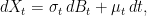(5)

the method can be applied. Now, the volatility in (3) is replaced by an average value across the interval (t_i-1, t_i).

The methods above are very useful, but there is a further improvement that can be made. Ideally, we would not have to specify an explicit value of the volatility σ. That is, it should be model independent. There are many reasons why this is desirable. Suppose that we are running a Monte Carlo simulation and generate samples of X at the times t_i. If the simulation only outputs values of X, then this is not sufficient to compute (3). So, it will be necessary to update the program running the simulation to also output the volatility. In some situations this might not be easy. For example, X could be a complicated function of various other processes and, although we could use Ito’s lemma to compute the volatility of X from the other processes, it could be messy. In some situations we might not even have access to the volatility or any method of computing it. For example, the values of X could be computed from historical data. We could be looking at the probability of stock prices crossing a level by looking at historical close fixings, without access to the complete intra-day data. In any case, a model independent discrete barrier adjustment would make applying it much easier.

Removing Volatility Dependence

How can the volatility term be removed from adjustment (3)? One idea is to replace it by an estimator computed from the samples of X, such as

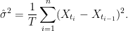$\displaystyle \hat\sigma^2=\frac1T\sum_{i=1}^n(X_{t_i}-X_{t_{i-1}})^2.$

While this would work, at least for a constant volatility process, it does not meet the requirements. For a general Ito process (5) with stochastic volatility, using an estimator computed over the whole time interval [0, T] may not be a good approximation for the volatility at the time that the barrier is hit. A possible way around this is for the adjustment (3) applied at time t_i to only depend on a volatility estimator computed from samples near the time. This would be possible, although it is not clear what is the best way to select these times. Besides, an important point to note is that we do not need a good estimate of the volatility, since that is not the goal here.

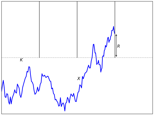
As explained in the previous post, adjustment (3) works because it corrects for the expected overshoot when the barrier is hit. Specifically, at the first time for which M_i ≥ K, the overshoot is R = X_t_i – K. If there was no adjustment then the overshoot is positive and the leading order term in the discrete barrier approximation error is proportional to 𝔼[R]. The positive shift added to X_t_i is chosen to compensate for this, giving zero expected overshoot to leading order, and reducing the barrier approximation error. The same applies to any similar adjustment. As long as there is sufficient freedom in choosing M_i, then it should be possible to do it in a way that has zero expected overshoot. Taking this to the extreme, it should be possible to compute the adjustment at time t_i using only the sampled values X_t_i-1 and X_t_i.

Consider adjustments of the form

$\displaystyle M_i=\theta(X_{t_{i-1}},X_{t_i})$

for θ: ℝ² → ℝ. By model independence, if this adjustment applies to a process X, then it should equally apply to the shifted and scaled processes X + a and bX for constants a and b > 0. Equivalently, θ satisfies the scaling and translation invariance,

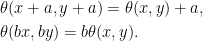$\displaystyle \begin{aligned} &\theta(x+a,y+a)=\theta(x,y)+a,\\ &\theta(bx,by)=b\theta(x,y). \end{aligned}$

(6)

This restricts the possible forms that θ can take.

Lemma 1 A function θ: ℝ² → ℝ satisfies (6) if and only if

$\displaystyle \theta(x,y)=py+(1-p)x+c\lvert y-x\rvert$

for constants p, c.

Proof: Write θ(0, u) as the sum of its antisymmetric and symmetric parts

$\displaystyle \theta(0,u)=(\theta(0,u)-\theta(0,-u))/2+(\theta(0,u)+\theta(0,-u))/2.$

By scaling invariance, the first term on the right is proportional to u and the second is proportional to |u|. Hence,

$\displaystyle \theta(0,u)=pu+c\lvert u\rvert$

for constants p and c. Using translation invariance,

$\displaystyle \begin{aligned} \theta(x,y) &= x + \theta(0,y-x)\\ &=x + p(y-x)+c\lvert y-x\rvert \end{aligned}$

as required. ⬜

I will therefore only consider adjustments where the maximum of the process across the interval (t_i-1, t_i) is replaced by

$\displaystyle M_i=pX_{t_i}+(1-p)X_{t_{i-1}}+c\lvert X_{t_i}-X_{t_{i-1}}\rvert.$

(7)

According to (3), the barrier condition sup_t≤TX_t ≥ K is replaced by the discrete approximation max_iM_i ≥ K.

There are various ways in which (7) can be parameterized, but this form is quite intuitive. The term pX_t_i + (1 - p)X_t_i-1 is an interpolation of the path of X, and c|X_t_i – X_t_i-1| represents a shift proportional to the sample deviation across the interval replacing the σ√δt term of the simple shift (3). The purpose of this post is to find values for p and c giving a good adjustment, improving convergence of the discrete approximation.

The discrete barrier condition M_i ≥ K given by (7) can be satisfied while the process is below the barrier level, giving a negative barrier ‘overshoot’ R = X_t_i – K as in figure 2. As we will see, this is vital to obtaining an accurate approximation for the hitting probability. Continue reading “Model-Independent Discrete Barrier Adjustments” →

Discrete Barrier Approximations

It is quite common to consider functions of real-time stochastic process which depend on whether or not it crosses a specified barrier level K. This can involve computing expectations involving a real-valued process X of the form

$\displaystyle V={\mathbb E}\left[f(X_T);\;\sup{}_{t\le T}X_t \ge K\right]$

(1)

for a positive time T and function f: ℝ → ℝ. I am using the notation 𝔼[A;S] to denote the expectation of random variable A restricted to event S, or 𝔼[A1_S].

One example is computing prices of financial derivatives such as barrier options, where T represents the expiration time and f is the payoff at expiry conditional on hitting upper barrier level K. A knock-in call option would have the final payoff f(x) = (x - a)₊ for a contractual strike of a. Knock-out options are similar, except that the payoff is conditioned on not hitting the barrier level. As the sum of knock-in and knock-out options is just an option with no barrier, both cases involve similar calculations.

Alternatively, the barrier can be discrete, meaning that it only involves sampling the process at a finite set of times 0 ≤ t₁ ≤ ⋯ ≤ t_n ≤ T. Then, equation (1) is replaced by

$\displaystyle V={\mathbb E}\left[f(X_T);\;\sup{}_{i=1,\ldots,n}X_{t_i}\ge K\right].$

(2)

Naturally, sampling at a finite set of times will reduce the probability of the barrier being reached and, so, if f is nonnegative then (2) will have a lower value than (1). It should still converge though as n goes to infinity and the sampling times become dense in the interval.

If the underlying process X is Brownian motion or geometric Brownian motion, possibly with a constant drift, then there are exact expressions for computing (1) in terms of integrating f against a normal density. See the post on the reflection principle for more information. However, it is difficult to find exact expressions for the discrete barrier (2) other than integrating over high-dimensional joint normal distributions. So, it can be useful to approximate a discrete barrier with analytic formulas for the continuous barrier. This is the idea used in the classic 1997 paper A Continuity Correction for Discrete Barrier Options by Broadie, Glasserman and Kou (freely available here).
We may want to compute the continuous barrier expectation (1) using Monte Carlo simulation. This is a common method, but involves generating sample paths of the process X at a finite set of times. This means that we are only able to sample at these times so, necessarily, are restricted to discrete barrier calculations as in (2).

I am primarily concerned with the second idea This is a very general issue, since Monte Carlo simulation is a common technique used in many applications. However, as it only represents sample paths at discrete time points, it necessarily involves discretely approximating continuous barrier levels. You may well ask why we would even want to use Monte Carlo if, as I mentioned above, there are exact expressions in these cases.In answer, such formulas only hold in very restrictive situations where the process X is a Brownian motion or geometric Brownian motion with constant drift. More generally it could be an ‘Ito process’ of the form

$\displaystyle dX_t=\sigma_t\,dB_t+\mu_t\,dt$

(3)

where B is standard Brownian motion. This describes X as a stochastic integral with respect to the predictable integrands σ and μ, which represent the volatility and drift of the process. Strictly speaking, these are ‘linear’ volatility and drift terms, rather than log-linear as used in many financial models applied to nonnegative processes such as stock prices. This is simply the choice made here, since this post is addressing a general mathematical problem of approximating continuous barriers and not restricting to such specific applications.

If the volatility and drift terms in (3) are not constant, then the exact formulas no longer hold. This is true, even if they are deterministic functions of time. In practice, these terms are often stochastic and can be rather general, in which case trying to find exact expressions is an almost hopeless task. Even though I concentrate on the case with constant volatility and drift in any calculations performed here, this is for convenience of exposition. The idea is that, as long as σ is piecewise continuous then, locally, it is well approximate as constant and the techniques discussed here should still apply.

In addition to considering general Ito processes (3), the ideas described here will apply to much more general functions of the process X than stated in (1). In the financial context, this means more general payoffs than simple knock-in or knock-out options. For example, autocallable trades involve a down-and-in put option but, additionally, contain a discrete set of upper barriers which cause the trade to make a final payment and terminate. They may also allow the issuer to early terminate the trade on a discrete set of dates. Furthermore, trades can depend on different assets with separate barriers on each of them, or on the average of a basket of assets, or have different barrier levels in different time periods. The list of possibilities is endless but, the idea is that each continuous barrier inside a complex payoff will be approximated by discretely sampled barrier conditions.

For efficiency, we may also want to approximate a discrete barrier with a large number of sampling times by one with fewer. The methods outlined in the post can also be used for this. In particular, the simple barrier shift described below could be used by taking the difference between the shift computed for the times actually sampled and the one for the required sample times. I do not go into details of this, but mention it now give an idea of the generality of the technique.

Figure 1: Discrete barrier approximation error

Let’s consider simply approximating a continuous barrier in (1) by the discrete barrier in (2). This will converge as the number of sampling times t_i increases but, the problem is, it converges very slowly. We can get an idea of the order of the error when the sampling times have a δt spacing which, with equally spaced times, is given by δt = T/n. This is as shown in figure 1 above. When the process first hits the continuous barrier level, it will be on average about δt/2 before the next sampling time. If X behaves approximately like a Brownian motion with volatiity σ over this interval then it will have about 50% chance of being above K at the next discrete time. On the other hand, it will be below K with about 50% probability, in which case with will drop a distance proportional to σ√δt below on average. This means that if the continuous barrier is hit, there is a probability roughly proportional to σ√δt that the discrete barrier is not hit. So, the error in approximating a continuous barrier (1) by the discrete case (2) is of the order of σ√δt which only tends to zero at rate 1/√n. Continue reading “Discrete Barrier Approximations” →

Continuous Semimartingales

A stochastic process is a semimartingale if and only if it can be decomposed as the sum of a local martingale and an FV process. This is stated by the Bichteler-Dellacherie theorem or, alternatively, is often taken as the definition of a semimartingale. For continuous semimartingales, which are the subject of this post, things simplify considerably. The terms in the decomposition can be taken to be continuous, in which case they are also unique. As usual, we work with respect to a complete filtered probability space ${(\Omega,\mathcal{F},\{\mathcal{F}_t\}_{t\ge0},{\mathbb P})}$ , all processes are real-valued, and two processes are considered to be the same if they are indistinguishable.

Theorem 1 A continuous stochastic process X is a semimartingale if and only if it decomposes as

$\displaystyle X=M+A$ (1)

for a continuous local martingale M and continuous FV process A. Furthermore, assuming that ${A_0=0}$ , decomposition (1) is unique.

Proof: As sums of local martingales and FV processes are semimartingales, X is a semimartingale whenever it satisfies the decomposition (1). Furthermore, if ${X=M+A=M^\prime+A^\prime}$ were two such decompositions with ${A_0=A^\prime_0=0}$ then ${M-M^\prime=A^\prime-A}$ is both a local martingale and a continuous FV process. Therefore, ${A^\prime-A}$ is constant, so ${A=A^\prime}$ and ${M=M^\prime}$ .

It just remains to prove the existence of decomposition (1). However, X is continuous and, hence, is locally square integrable. So, Lemmas 4 and 5 of the previous post say that we can decompose ${X=M+A}$ where M is a local martingale, A is an FV process and the quadratic covariation ${[M,A]}$ is a local martingale. As X is continuous we have ${\Delta M=-\Delta A}$ so that, by the properties of covariations,

$\displaystyle -[M,A]_t=-\sum_{s\le t}\Delta M_s\Delta A_s=\sum_{s\le t}(\Delta A_s)^2.$

(2)

We have shown that ${-[M,A]}$ is a nonnegative local martingale so, in particular, it is a supermartingale. This gives ${\mathbb{E}[-[M,A]_t]\le\mathbb{E}[-[M,A]_0]=0}$ . Then (2) implies that ${\Delta A}$ is zero and, hence, A and ${M=X-A}$ are continuous. ⬜

Using decomposition (1), it can be shown that a predictable process ${\xi}$ is X-integrable if and only if it is both M-integrable and A-integrable. Then, the integral with respect to X breaks down into the sum of the integrals with respect to M and A. This greatly simplifies the construction of the stochastic integral for continuous semimartingales. The integral with respect to the continuous FV process A is equivalent to Lebesgue-Stieltjes integration along sample paths, and it is possible to construct the integral with respect to the continuous local martingale M for the full set of M-integrable integrands using the Ito isometry. Many introductions to stochastic calculus focus on integration with respect to continuous semimartingales, which is made much easier because of these results.

Theorem 2 Let ${X=M+A}$ be the decomposition of the continuous semimartingale X into a continuous local martingale M and continuous FV process A. Then, a predictable process ${\xi}$ is X-integrable if and only if

$\displaystyle \int_0^t\xi^2\,d[M]+\int_0^t\vert\xi\vert\,\vert dA\vert < \infty$ (3)

almost surely, for each time ${t\ge0}$ . In that case, ${\xi}$ is both M-integrable and A-integrable and,

$\displaystyle \int\xi\,dX=\int\xi\,dM+\int\xi\,dA$ (4)

gives the decomposition of ${\int\xi\,dX}$ into its local martingale and FV terms.

Continue reading “Continuous Semimartingales” →

	Anonymous on Spitzer’s Formula
	Anonymous on Spitzer’s Formula
	Anonymous on Brownian Bridges
	Anonymous on Spitzer’s Formula
	Anonymous on Spitzer’s Formula
	Anonymous on Spitzer’s Formula
	Anonymous on Spitzer’s Formula
	Anonymous on Spitzer’s Formula
	Anonymous on Spitzer’s Formula
	Anonymous on Spitzer’s Formula