For nonnegative local martingales, there is an interesting symmetry between the failure of the martingale property and the possibility of hitting zero, which I will describe now. I will also give a necessary and sufficient condition for solutions to a certain class of stochastic differential equations to hit zero in finite time and, using the aforementioned symmetry, infer a necessary and sufficient condition for the processes to be proper martingales. It is often the case that solutions to SDEs are clearly local martingales, but is hard to tell whether they are proper martingales. So, the martingale condition, given in Theorem 4 below, is a useful result to know. The method described here is relatively new to me, only coming up while preparing the previous post. Applying a hedging argument, it was noted that the failure of the martingale property for solutions to the SDE  for
for  is related to the fact that, for
  , the process hits zero. This idea extends to all continuous and nonnegative local martingales. The Girsanov transform method applied here is essentially the same as that used by Carlos A. Sin (Complications with stochastic volatility models, Adv. in Appl. Probab. Volume 30, Number 1, 1998, 256-268) and B. Jourdain (Loss of martingality in asset price models with lognormal stochastic volatility, Preprint CERMICS, 2004-267).
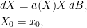
Consider nonnegative solutions to the stochastic differential equation
 |
(1) |
where  , B is a Brownian motion and the fixed initial condition
  is strictly positive. The multiplier X in the coefficient of dB ensures that if X ever hits zero then it stays there. By time-change methods, uniqueness in law is guaranteed as long as a is nonzero and
  is locally integrable on
  . Consider also the following SDE,
 |
(2) |
Being integrals with respect to Brownian motion, solutions to (1) and (2) are local martingales. It is possible for them to fail to be proper martingales though, and they may or may not hit zero at some time. These possibilities are related by the following result.
Theorem 1 Suppose that (1) and (2) satisfy uniqueness in law. Then, X is a proper martingale if and only if Y never hits zero. Similarly, Y is a proper martingale if and only if X never hits zero.
As an example, consider  for some fixed exponent
  , so that
  . In the previous post it was shown that X fails to be a proper martingale when
  and hits zero when
  . Theorem 1 shows that these two statements are equivalent.
We can be a bit more precise than the statement in Theorem 1. Being nonnegative local martingales, the processes X, Y are automatically supermartingales. For times  ,
, ![{X_s-{\mathbb E}[X_t\mid\mathcal{F}_s]}](https://s0.wp.com/latex.php?latex=%7BX_s-%7B%5Cmathbb+E%7D%5BX_t%5Cmid%5Cmathcal%7BF%7D_s%5D%7D&bg=ffffff&fg=000000&s=0&c=20201002) is nonnegative and, hence, will be almost surely zero if and only if it has zero expectation. So, we see that the martingale condition
is nonnegative and, hence, will be almost surely zero if and only if it has zero expectation. So, we see that the martingale condition ![{X_s={\mathbb E}[X_t\mid\mathcal{F}_s]}](https://s0.wp.com/latex.php?latex=%7BX_s%3D%7B%5Cmathbb+E%7D%5BX_t%5Cmid%5Cmathcal%7BF%7D_s%5D%7D&bg=ffffff&fg=000000&s=0&c=20201002) is satisfied whenever
is satisfied whenever ![{{\mathbb E}[X_s]={\mathbb E}[X_t]}](https://s0.wp.com/latex.php?latex=%7B%7B%5Cmathbb+E%7D%5BX_s%5D%3D%7B%5Cmathbb+E%7D%5BX_t%5D%7D&bg=ffffff&fg=000000&s=0&c=20201002) . Furthermore, the supermartingale condition gives
. Furthermore, the supermartingale condition gives ![{x_0\ge{\mathbb E}[X_s]\ge{\mathbb E}[X_t]}](https://s0.wp.com/latex.php?latex=%7Bx_0%5Cge%7B%5Cmathbb+E%7D%5BX_s%5D%5Cge%7B%5Cmathbb+E%7D%5BX_t%5D%7D&bg=ffffff&fg=000000&s=0&c=20201002) . It follows that X is a martingale over a time interval
. It follows that X is a martingale over a time interval ![{[0,t]}](https://s0.wp.com/latex.php?latex=%7B%5B0%2Ct%5D%7D&bg=ffffff&fg=000000&s=0&c=20201002) if and only if
if and only if ![{{\mathbb E}[X_t]=x_0}](https://s0.wp.com/latex.php?latex=%7B%7B%5Cmathbb+E%7D%5BX_t%5D%3Dx_0%7D&bg=ffffff&fg=000000&s=0&c=20201002) . The following theorem shows that this is equivalent to
. The following theorem shows that this is equivalent to  being strictly positive with probability one, giving a more precise statement than Theorem 1 above.
Theorem 2 Suppose that (1) and (2) satisfy uniqueness in law. Then,
![\displaystyle \setlength\arraycolsep{2pt} \begin{array}{rl} &\displaystyle{\mathbb E}[X_t]=x_0{\mathbb P}(Y_t>0),\smallskip\\ &\displaystyle{\mathbb E}[Y_t]=y_0{\mathbb P}(X_t>0). \end{array}](https://s0.wp.com/latex.php?latex=%5Cdisplaystyle++%5Csetlength%5Carraycolsep%7B2pt%7D+%5Cbegin%7Barray%7D%7Brl%7D+%26%5Cdisplaystyle%7B%5Cmathbb+E%7D%5BX_t%5D%3Dx_0%7B%5Cmathbb+P%7D%28Y_t%3E0%29%2C%5Csmallskip%5C%5C+%26%5Cdisplaystyle%7B%5Cmathbb+E%7D%5BY_t%5D%3Dy_0%7B%5Cmathbb+P%7D%28X_t%3E0%29.+%5Cend%7Barray%7D+&bg=ffffff&fg=000000&s=0&c=20201002) |
(3) |
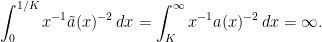
To apply these results, the following necessary and sufficient condition for solutions to the SDE (1) to hit zero after a finite time can be used. This is a special case of Feller’s test for explosions, and a proof is given further below.
Theorem 3 Suppose that a is nonzero and is locally integrable on . Then, solutions X to (1) hit zero with positive probability if and only if
 |
(4) |
for  . In this case, X hits zero almost surely.
Using Theorem 1, this can be transformed into a condition for the process X to be a martingale. In particular, X satisfying (1) will be a proper martingale if and only if the solution Y to (2) has zero probability of hitting zero. By Theorem 3 this is equivalent to
So, we have arrived at a necessary and sufficient condition for X to be a martingale.
Theorem 4 Suppose that a is nonzero and is locally integrable on . Then, solutions X to (1) are proper martingales if and only if
 |
(5) |
for .
Looking again at the SDE , we take  ,
,
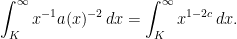
This is infinite if and only if  , in which case X is a martingale and, for , Theorem 4 shows that it fails to be a martingale. Consider, also, the following SDE, whose coefficient grows very slightly faster than linearly in X,
 |
(6) |
Again, c is a fixed positive constant. In this case, we take  . Up to a finite scaling factor, the integral (4) gives
![\displaystyle \setlength\arraycolsep{2pt} \begin{array}{rl} \displaystyle\int_K^\infty x^{-1}a(x)^{-2}\,dx&\displaystyle\sim\int_K^\infty x^{-1}(\log x)^{-2c}\,dx\smallskip\\ &\displaystyle=\begin{cases} (1-2c)^{-1}\left[(\log x)^{1-2c}\right]_K^\infty,&\textrm{if }c\not=1/2,\\ \left[\log\log x\right]_K^\infty,&\textrm{if }c=1/2. \end{cases} \end{array}](https://s0.wp.com/latex.php?latex=%5Cdisplaystyle++%5Csetlength%5Carraycolsep%7B2pt%7D+%5Cbegin%7Barray%7D%7Brl%7D+%5Cdisplaystyle%5Cint_K%5E%5Cinfty+x%5E%7B-1%7Da%28x%29%5E%7B-2%7D%5C%2Cdx%26%5Cdisplaystyle%5Csim%5Cint_K%5E%5Cinfty+x%5E%7B-1%7D%28%5Clog+x%29%5E%7B-2c%7D%5C%2Cdx%5Csmallskip%5C%5C+%26%5Cdisplaystyle%3D%5Cbegin%7Bcases%7D+%281-2c%29%5E%7B-1%7D%5Cleft%5B%28%5Clog+x%29%5E%7B1-2c%7D%5Cright%5D_K%5E%5Cinfty%2C%26%5Ctextrm%7Bif+%7Dc%5Cnot%3D1%2F2%2C%5C%5C+%5Cleft%5B%5Clog%5Clog+x%5Cright%5D_K%5E%5Cinfty%2C%26%5Ctextrm%7Bif+%7Dc%3D1%2F2.+%5Cend%7Bcases%7D+%5Cend%7Barray%7D+&bg=ffffff&fg=000000&s=0&c=20201002)
This is finite if and only if  . So, solutions to (6) are martingales whenever
  and are local martingales, but not proper martingales, for all .
Proof of Theorem 2
I will now give a proof of Theorem 2 using local Girsanov transforms. As is standard, we work with respect to a filtered probability space 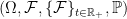 . However, in order for the Girsanov transform method to be successfully applied, we do not assume that the filtration is complete. We will also work in the more general setting of continuous local martingales, not necessarily defined by an SDE.
For the remainder of this section, let X be a continuous local martingale taking values in the extended nonnegative real numbers ![{\bar{\mathbb R}_+=[0,\infty]}](https://s0.wp.com/latex.php?latex=%7B%5Cbar%7B%5Cmathbb+R%7D_%2B%3D%5B0%2C%5Cinfty%5D%7D&bg=ffffff&fg=000000&s=0&c=20201002) , and with the fixed initial condition
, and with the fixed initial condition  . The local martingale property implies that X is a supermartingale and that it is almost surely finite. Let us also set
  and Y=1/X, which explodes when X hits zero and hits zero in the (zero probability) event that X explodes. Let also define
  to be the first time at which X hits zero and
  to be the first time at which Y hits zero or, equivalently, X hits infinity. From this setup, is almost-surely infinite.
The idea is to use X to define a change of measure 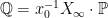 . However, Girsanov transform theory would only be applicable when X is a uniformly integrable and positive martingale. To get around this restriction, we instead apply the change of measure locally. That is, if
  is a stopping time such that
  is a uniformly integrable martingale and
  , then we define the restriction of the probability measure
  to
to  by
by
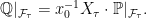 |
(7) |
That is, ![{{\mathbb E}_{\mathbb Q}[Z]=x_0^{-1}{\mathbb E}[X_\tau Z]}](https://s0.wp.com/latex.php?latex=%7B%7B%5Cmathbb+E%7D_%7B%5Cmathbb+Q%7D%5BZ%5D%3Dx_0%5E%7B-1%7D%7B%5Cmathbb+E%7D%5BX_%5Ctau+Z%5D%7D&bg=ffffff&fg=000000&s=0&c=20201002) for any bounded -measurable random variable Z. There is a subtle issue here though, as the measure need not exist at all. This is an issue which was encountered previously in my stochastic calculus notes, in the application of measure changes to stochastic differential equations. This problem can arise because, although
for any bounded -measurable random variable Z. There is a subtle issue here though, as the measure need not exist at all. This is an issue which was encountered previously in my stochastic calculus notes, in the application of measure changes to stochastic differential equations. This problem can arise because, although  and are defined to be equivalent on , they need not be equivalent on
  . For example, being a local martingale, X is almost surely bounded under . However, if it is not a proper martingale, then we will see that Y=1/X hits zero in a finite time, at which X explodes. If we did not include such events in the probability space to start with, then defining the transformed measure would be impossible. Similarly, problems would be caused by including such zero probability events in the initial sigma algebra
  . This is the reason for considering X to lie in the extended nonnegative real numbers in the setup above, and also for not assuming that the filtration satisfies the usual completeness properties. These are not real problems though, and just require a bit of care with the construction of the underlying filtered probability space. For now, we ignore these issues and assume that the measure exists, in which case it is essentially unique. We can prove the following much more general version of Theorem 2, applying to arbitrary continuous and nonnegative local martingales. Actually, Theorem 2 will follow as a corollary of Lemma 5 when applied to solutions of the SDE (1).
Lemma 5 If it exists, the measure defined by (7) is uniquely defined on  . Furthermore,
  ,
,  is a -local martingale with quadratic variation
![\displaystyle [\tilde Y]_t=\int_0^{t\wedge\tau_Y} X^{-4}\,d[X]](https://s0.wp.com/latex.php?latex=%5Cdisplaystyle++%5B%5Ctilde+Y%5D_t%3D%5Cint_0%5E%7Bt%5Cwedge%5Ctau_Y%7D+X%5E%7B-4%7D%5C%2Cd%5BX%5D+&bg=ffffff&fg=000000&s=0&c=20201002) |
(8) |
(under ) and, for any time  ,
,
![\displaystyle \setlength\arraycolsep{2pt} \begin{array}{rl} &\displaystyle{\mathbb E}_{\mathbb P}[X_t]=x_0{\mathbb Q}(\tilde Y_t>0),\smallskip\\ &\displaystyle{\mathbb E}_{\mathbb Q}[\tilde Y_t]=y_0{\mathbb P}(X_t>0). \end{array}](https://s0.wp.com/latex.php?latex=%5Cdisplaystyle++%5Csetlength%5Carraycolsep%7B2pt%7D+%5Cbegin%7Barray%7D%7Brl%7D+%26%5Cdisplaystyle%7B%5Cmathbb+E%7D_%7B%5Cmathbb+P%7D%5BX_t%5D%3Dx_0%7B%5Cmathbb+Q%7D%28%5Ctilde+Y_t%3E0%29%2C%5Csmallskip%5C%5C+%26%5Cdisplaystyle%7B%5Cmathbb+E%7D_%7B%5Cmathbb+Q%7D%5B%5Ctilde+Y_t%5D%3Dy_0%7B%5Cmathbb+P%7D%28X_t%3E0%29.+%5Cend%7Barray%7D+&bg=ffffff&fg=000000&s=0&c=20201002) |
(9) |
Proof: Let  be a sequence of stopping times increasing to
  and such that
  are uniformly integrable martingales with
  (almost surely). For example, we could take to be the first time that X hits either n or 1/n. Then, (7) defines the restriction of to
  . Letting n go to infinity this uniquely defines on
  . Once it is shown that
  -almost surely, then this will also uniquely determine on .
By Ito’s lemma,
![\displaystyle dY=\frac{-1}{X^2}\,dX+\frac{1}{X^3}\,d[X],](https://s0.wp.com/latex.php?latex=%5Cdisplaystyle++dY%3D%5Cfrac%7B-1%7D%7BX%5E2%7D%5C%2CdX%2B%5Cfrac%7B1%7D%7BX%5E3%7D%5C%2Cd%5BX%5D%2C+&bg=ffffff&fg=000000&s=0&c=20201002) |
(10) |
so that ![{d[Y]=X^{-4}\,d[X]}](https://s0.wp.com/latex.php?latex=%7Bd%5BY%5D%3DX%5E%7B-4%7D%5C%2Cd%5BX%5D%7D&bg=ffffff&fg=000000&s=0&c=20201002) and
and ![{d[X,Y]=-X^{-2}\,d[X]}](https://s0.wp.com/latex.php?latex=%7Bd%5BX%2CY%5D%3D-X%5E%7B-2%7D%5C%2Cd%5BX%5D%7D&bg=ffffff&fg=000000&s=0&c=20201002) . However, applying the Girsanov theorem to the local martingale X shows that
. However, applying the Girsanov theorem to the local martingale X shows that
![\displaystyle M\equiv X-\int X^{-1}\,d[X]](https://s0.wp.com/latex.php?latex=%5Cdisplaystyle++M%5Cequiv+X-%5Cint+X%5E%7B-1%7D%5C%2Cd%5BX%5D+&bg=ffffff&fg=000000&s=0&c=20201002)
is a -local martingale over the intervals ![{[0,\tau_n]}](https://s0.wp.com/latex.php?latex=%7B%5B0%2C%5Ctau_n%5D%7D&bg=ffffff&fg=000000&s=0&c=20201002) and, therefore, so is
and, therefore, so is  . Letting n go to infinity shows that
  is a -local martingale. In particular, by the supermartingale property,
 ![{{\mathbb E}_{\mathbb Q}[Y_{\tau_X\wedge\tau_Y}]\le y_0<\infty}](https://s0.wp.com/latex.php?latex=%7B%7B%5Cmathbb+E%7D_%7B%5Cmathbb+Q%7D%5BY_%7B%5Ctau_X%5Cwedge%5Ctau_Y%7D%5D%5Cle+y_0%3C%5Cinfty%7D&bg=ffffff&fg=000000&s=0&c=20201002) so that
so that  is finite and -almost surely.
So, we have shown that , is uniquely defined on and that  is a -local martingale. Using (10), the quadratic variation of Y is given by
![\displaystyle d[Y]=\frac{1}{X^4}\,d[X]](https://s0.wp.com/latex.php?latex=%5Cdisplaystyle++d%5BY%5D%3D%5Cfrac%7B1%7D%7BX%5E4%7D%5C%2Cd%5BX%5D+&bg=ffffff&fg=000000&s=0&c=20201002)
on ![{[0,\tau_X\wedge\tau_Y]}](https://s0.wp.com/latex.php?latex=%7B%5B0%2C%5Ctau_X%5Cwedge%5Ctau_Y%5D%7D&bg=ffffff&fg=000000&s=0&c=20201002) , giving (8).
, giving (8).
The first of the identities in (9) comes from the following sequence of equalities.
![\displaystyle \setlength\arraycolsep{2pt} \begin{array}{rl} \displaystyle{\mathbb Q}(\tilde Y_t>0)&\displaystyle=\lim_{n\rightarrow\infty}{\mathbb Q}(\tau_n>t)\smallskip\\ &\displaystyle=\lim_{n\rightarrow\infty}x_0^{-1}{\mathbb E}[X_{\tau_n}1_{\{\tau_n>t\}}]\smallskip\\ &\displaystyle=x_0^{-1}{\mathbb E}[X_t1_{\{\tau_X>t\}}]=x_0^{-1}{\mathbb E}[X_t]. \end{array}](https://s0.wp.com/latex.php?latex=%5Cdisplaystyle++%5Csetlength%5Carraycolsep%7B2pt%7D+%5Cbegin%7Barray%7D%7Brl%7D+%5Cdisplaystyle%7B%5Cmathbb+Q%7D%28%5Ctilde+Y_t%3E0%29%26%5Cdisplaystyle%3D%5Clim_%7Bn%5Crightarrow%5Cinfty%7D%7B%5Cmathbb+Q%7D%28%5Ctau_n%3Et%29%5Csmallskip%5C%5C+%26%5Cdisplaystyle%3D%5Clim_%7Bn%5Crightarrow%5Cinfty%7Dx_0%5E%7B-1%7D%7B%5Cmathbb+E%7D%5BX_%7B%5Ctau_n%7D1_%7B%5C%7B%5Ctau_n%3Et%5C%7D%7D%5D%5Csmallskip%5C%5C+%26%5Cdisplaystyle%3Dx_0%5E%7B-1%7D%7B%5Cmathbb+E%7D%5BX_t1_%7B%5C%7B%5Ctau_X%3Et%5C%7D%7D%5D%3Dx_0%5E%7B-1%7D%7B%5Cmathbb+E%7D%5BX_t%5D.+%5Cend%7Barray%7D+&bg=ffffff&fg=000000&s=0&c=20201002)
The first equality is using the fact that, -almost surely, Y hits zero at time  whenever this is finite. The second equality is just using the change of measure definition (7). The third equality is using the condition that are martingales and
  -almost surely. In a similar way, the second of the identities in (9) comes from the following,
![\displaystyle \setlength\arraycolsep{2pt} \begin{array}{rl} \displaystyle{\mathbb E}_{\mathbb Q}[\tilde Y_t]&\displaystyle=\lim_{n\rightarrow\infty}{\mathbb E}_{\mathbb Q}[Y_t 1_{\{\tau_n>t\}}]\smallskip\\ &=\lim_{n\rightarrow\infty}x_0^{-1}{\mathbb E}[X_{\tau_n}Y_t1_{\{\tau_n>t\}}]\smallskip\\ &\displaystyle=x_0^{-1}{\mathbb E}[X_tY_t1_{\{\tau_X>t\}}]=x_0^{-1}{\mathbb P}(X_t>0). \end{array}](https://s0.wp.com/latex.php?latex=%5Cdisplaystyle++%5Csetlength%5Carraycolsep%7B2pt%7D+%5Cbegin%7Barray%7D%7Brl%7D+%5Cdisplaystyle%7B%5Cmathbb+E%7D_%7B%5Cmathbb+Q%7D%5B%5Ctilde+Y_t%5D%26%5Cdisplaystyle%3D%5Clim_%7Bn%5Crightarrow%5Cinfty%7D%7B%5Cmathbb+E%7D_%7B%5Cmathbb+Q%7D%5BY_t+1_%7B%5C%7B%5Ctau_n%3Et%5C%7D%7D%5D%5Csmallskip%5C%5C+%26%3D%5Clim_%7Bn%5Crightarrow%5Cinfty%7Dx_0%5E%7B-1%7D%7B%5Cmathbb+E%7D%5BX_%7B%5Ctau_n%7DY_t1_%7B%5C%7B%5Ctau_n%3Et%5C%7D%7D%5D%5Csmallskip%5C%5C+%26%5Cdisplaystyle%3Dx_0%5E%7B-1%7D%7B%5Cmathbb+E%7D%5BX_tY_t1_%7B%5C%7B%5Ctau_X%3Et%5C%7D%7D%5D%3Dx_0%5E%7B-1%7D%7B%5Cmathbb+P%7D%28X_t%3E0%29.+%5Cend%7Barray%7D+&bg=ffffff&fg=000000&s=0&c=20201002)
⬜
Now, let’s move on to showing that with the underlying filtered probability space set up correctly, measures defined by local Girsanov transforms do indeed exist. The idea is to construct locally via equation (7), and apply the Kolmogorov extension theorem to extend to a measure on  . Kolmogorov’s theorem states that if we have a consistent set of probability measures defined on the finite products of some underlying measurable spaces (in particular, Polish spaces), then they extend uniquely to a measure on the infinite product.
Lemma 6 Let  be the set of continuous functions
  , X be the coordinate process

 be the natural filtration

and set  .
.
Then, for any probability measure on making X a local martingale with  almost surely, a measure defined by (7) exists.
Proof: Let each n, let be the stopping time

These increase to a limit  , which is the first time that X hits either zero or infinity. Define the measure
  on
on  according to (7),

This can be extended to a measure on the sigma algebra by supposing that X remains constant after time . That is, the -expectation of any -measurable and bounded function  is given by,
![\displaystyle {\mathbb E}_{{\mathbb Q}^n}[F(X)]=x_0^{-1}{\mathbb E}\left[X_{\tau_n}F(X^{\tau_n})\right].](https://s0.wp.com/latex.php?latex=%5Cdisplaystyle++%7B%5Cmathbb+E%7D_%7B%7B%5Cmathbb+Q%7D%5En%7D%5BF%28X%29%5D%3Dx_0%5E%7B-1%7D%7B%5Cmathbb+E%7D%5Cleft%5BX_%7B%5Ctau_n%7DF%28X%5E%7B%5Ctau_n%7D%29%5Cright%5D.+&bg=ffffff&fg=000000&s=0&c=20201002)
This defines a sequence of measures on such that, for all  ,
,  and agree when restricted to
  . Denote the infinite product space as
  with product sigma algebra
  , and let
  be the projection onto the n‘th component. Then, applying the Kolmogorov extension theorem, there exists a measure
  on
on  with respect to which has distribution and, for any ,
  and are equal up until the first time that they exceed the level m or drop below 1/m, -almost surely. With respect to , then, the limit
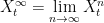
exists and, up until the first time at which it passes the upper level n or drops below 1/n, this agrees with the distrubution of X under the measure . It can also be seen that  is almost surely continuous. So, we can define to be the measure on with respect to which X has the same distribution as does under . Finally, for a stopping time for which is a -uniformly integrable martingale and , it needs to be shown that (7) holds. For any finite time t and bounded
  -measurable random variable Z,
  is -measurable. So, using the martingale property for X,
![\displaystyle \setlength\arraycolsep{2pt} \begin{array}{rl} \displaystyle{\mathbb E}_{{\mathbb Q}}[Z1_{\{\tau_\infty>\tau\wedge t\}}]&\displaystyle=\lim_{n\rightarrow\infty}{\mathbb E}_{\mathbb Q}[Z1_{\{\tau_n>\tau\wedge t\}}]\smallskip\\ &\displaystyle=\lim_{n\rightarrow\infty}x_0^{-1}{\mathbb E}[X_{\tau_n}Z1_{\{\tau_n>\tau\wedge t\}}]\smallskip\\ &\displaystyle=x_0^{-1}{\mathbb E}[X_{\tau}Z]. \end{array}](https://s0.wp.com/latex.php?latex=%5Cdisplaystyle++%5Csetlength%5Carraycolsep%7B2pt%7D+%5Cbegin%7Barray%7D%7Brl%7D+%5Cdisplaystyle%7B%5Cmathbb+E%7D_%7B%7B%5Cmathbb+Q%7D%7D%5BZ1_%7B%5C%7B%5Ctau_%5Cinfty%3E%5Ctau%5Cwedge+t%5C%7D%7D%5D%26%5Cdisplaystyle%3D%5Clim_%7Bn%5Crightarrow%5Cinfty%7D%7B%5Cmathbb+E%7D_%7B%5Cmathbb+Q%7D%5BZ1_%7B%5C%7B%5Ctau_n%3E%5Ctau%5Cwedge+t%5C%7D%7D%5D%5Csmallskip%5C%5C+%26%5Cdisplaystyle%3D%5Clim_%7Bn%5Crightarrow%5Cinfty%7Dx_0%5E%7B-1%7D%7B%5Cmathbb+E%7D%5BX_%7B%5Ctau_n%7DZ1_%7B%5C%7B%5Ctau_n%3E%5Ctau%5Cwedge+t%5C%7D%7D%5D%5Csmallskip%5C%5C+%26%5Cdisplaystyle%3Dx_0%5E%7B-1%7D%7B%5Cmathbb+E%7D%5BX_%7B%5Ctau%7DZ%5D.+%5Cend%7Barray%7D+&bg=ffffff&fg=000000&s=0&c=20201002) |
(11) |
The last equality here uses the martingale property to replace  by
by  , and the fact that
  for large n, almost surely, which follows from the property that is almost surely bounded and nonzero. Using Z=1 in (11) shows that
  -almost surely and, letting t increase to infinity,
![\displaystyle {\mathbb E}_{\mathbb Q}[Z]=x_0^{-1}{\mathbb E}[X_\tau Z]](https://s0.wp.com/latex.php?latex=%5Cdisplaystyle++%7B%5Cmathbb+E%7D_%7B%5Cmathbb+Q%7D%5BZ%5D%3Dx_0%5E%7B-1%7D%7B%5Cmathbb+E%7D%5BX_%5Ctau+Z%5D+&bg=ffffff&fg=000000&s=0&c=20201002)
for all -measurable and bounded random variables Z. ⬜
Now that it has been shown that the measure change is well-defined, assuming the setup of Lemma 6, we can finally move on to the proof of Theorem 2. Rather than defining the process X via the SDE (1), however, it helps to rewrite it in a more intrinsic form without reference to a driving Brownian motion. Any such process is a local martingale with quadratic variation
![\displaystyle [X]_t=\int_0^t a(X_s)^2X_s^2\,ds.](https://s0.wp.com/latex.php?latex=%5Cdisplaystyle++%5BX%5D_t%3D%5Cint_0%5Et+a%28X_s%29%5E2X_s%5E2%5C%2Cds.+&bg=ffffff&fg=000000&s=0&c=20201002) |
(12) |
Conversely, by enlarging the probability space to add a Brownian motion if required, any local martingale satisfying (12) and the initial condition solves the SDE (\ref) for some Brownian motion B}. So, assuming uniqueness in law of (2), Theorem 2 is a consequence of equations (9) and the following result.
Lemma 7 Assume the setup of Lemma (6) and let be a probability measure on with respect to which X is a local martingale satisfying almost surely, and with quadratic variation given by (12).
Then, letting be the measure defined by Lemma 5, the process  is a -local martingale with quadratic variation
![\displaystyle [\tilde Y]_t=\int_0^ta(\tilde Y^{-1}_s)^2\tilde Y_s^2\,ds.](https://s0.wp.com/latex.php?latex=%5Cdisplaystyle++%5B%5Ctilde+Y%5D_t%3D%5Cint_0%5Eta%28%5Ctilde+Y%5E%7B-1%7D_s%29%5E2%5Ctilde+Y_s%5E2%5C%2Cds.+&bg=ffffff&fg=000000&s=0&c=20201002) |
(13) |
Proof: Lemma 5 states that is a -local martingale with quadratic variation
![\displaystyle \setlength\arraycolsep{2pt} \begin{array}{rl} \displaystyle[\tilde Y]_t&\displaystyle=\int_0^{t\wedge\tau_Y}X_s^{-4}\,d[X]_s\smallskip\\ &\displaystyle=\int_0^{t\wedge\tau_Y}X_s^{-4}a(X_s)^2X_s^2\,ds\smallskip\\ &\displaystyle=\int_0^{t\wedge\tau_Y}a(\tilde Y^{-1}_s)^2\tilde Y_s^2\,ds. \end{array}](https://s0.wp.com/latex.php?latex=%5Cdisplaystyle++%5Csetlength%5Carraycolsep%7B2pt%7D+%5Cbegin%7Barray%7D%7Brl%7D+%5Cdisplaystyle%5B%5Ctilde+Y%5D_t%26%5Cdisplaystyle%3D%5Cint_0%5E%7Bt%5Cwedge%5Ctau_Y%7DX_s%5E%7B-4%7D%5C%2Cd%5BX%5D_s%5Csmallskip%5C%5C+%26%5Cdisplaystyle%3D%5Cint_0%5E%7Bt%5Cwedge%5Ctau_Y%7DX_s%5E%7B-4%7Da%28X_s%29%5E2X_s%5E2%5C%2Cds%5Csmallskip%5C%5C+%26%5Cdisplaystyle%3D%5Cint_0%5E%7Bt%5Cwedge%5Ctau_Y%7Da%28%5Ctilde+Y%5E%7B-1%7D_s%29%5E2%5Ctilde+Y_s%5E2%5C%2Cds.+%5Cend%7Barray%7D+&bg=ffffff&fg=000000&s=0&c=20201002)
As  after time , this gives (13). ⬜
Proof of the zero-hitting condition
Theorem 3, providing a necessary and sufficient condition for solutions to the SDE (1) to hit zero, can be proven by applying a well-chosen transformation to the local martingale X. Then, martingale convergence will be used — with probability one, whenever a continuous local martingale is bounded above or below then it converges to a finite value as  . The result also follows from Feller’s test for explosions (see Karatzas and Shreve, Brownian Motion and Stochastic Calculus, Chapter 5).
As is assumed to be locally integrable, a convex function  can be defined by
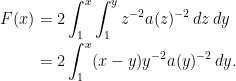
This is continuously differentiable with second order derivative  defined in the sense of distributions. Ito’s lemma gives
![\displaystyle F(X)=F(x_0)+\int F^\prime(X)\,dX+\int X^{-2}a(X)^{-2}\,d[X].](https://s0.wp.com/latex.php?latex=%5Cdisplaystyle++F%28X%29%3DF%28x_0%29%2B%5Cint+F%5E%5Cprime%28X%29%5C%2CdX%2B%5Cint+X%5E%7B-2%7Da%28X%29%5E%7B-2%7D%5C%2Cd%5BX%5D.+&bg=ffffff&fg=000000&s=0&c=20201002) |
(14) |
Although Ito’s lemma only directly applies in the twice differentiable case, where a is continuous, (14) extends to all a with locally integrable by taking limits (using the dominated convergence theorem to take the limits, and the monotone class theorem to extend to locally integrable). Then, as X satisfies the SDE (1) and a is assumed to be nonzero, its quadratic variation is given by ![{d[X]=a(X)^2X^2\,dt}](https://s0.wp.com/latex.php?latex=%7Bd%5BX%5D%3Da%28X%29%5E2X%5E2%5C%2Cdt%7D&bg=ffffff&fg=000000&s=0&c=20201002) for
for  nonzero up until the time at which X hits zero. So

where is the first time at which X hits zero. In particular,  is a local martingale. The limiting value of F at zero is

which is just the integral (4). If this is infinite, X cannot hit zero in finite time, as it would imply that the local martingale M explodes. Alternatively, suppose that the integral (4) is finite, so that  is finite. As X is a nonnegative local martingale, it converges almost surely to a finite value at infinity. So,
  is bounded above and, by martingale convergence, tends to a finite limit. This shows that
  converges as , which can only be the case if is finite and X hits zero.

This symmetry idea of linking the martingale property of one diffusion process to the explosion behavior of another diffusion process is very interesting. I think the Theorem 4 here coincides the Theorem 1.1 in this paper: .
Two follow-up questions: (1) Can we extend the result to one dimensional time-inhomogeneous diffusion?
(2) How about Doleans-Dade stochastic exponentials? Is there a similar result that exhibit this symmetry?
btw, I find all your posts very helpful for understanding stochastic calculus~ 🙂
Sorry, the link I refer to is: ” http://homepage.alice.de/murusov/papers/cev.pdf“.
Thanks, that’s an interesting reference and certainly very relevant to this post. Their Theorem 1.1 is exactly the same as my Theorem 4.
To answer (1), there is no problem in extending the ideas in this post to time-inhomogeneous diffusions. In fact, I was originally going to state Theorem 1 in this greater generality, but it didn’t seem to gain a lot and maybe would lose a bit of clarity. The proof I give (section “Proof of Theorem 2”) does not rely on it being a diffusion, so similar statements can be given for all continuous nonnegative local martingales (i.e., X is a proper martingale iff Y never hits zero).
The main statement for one dimensional diffusions, Theorem 4, does rely on time-homogenity because in that case we have a simple condition for zero-hitting, and therefore a simple condition for loss of the martingale property.
For (2), are you thinking about conditions for the Doleans exponential of a local martingale M to be a proper martingale? You can certain apply the method used here to it, although I’m not sure how useful a condition you obtain. I’d have to think about that a bit more.
Thank you for your prompt reply! Yes, I mean that form for the Q(2).
Also on the issue of linking “loss of martingale property” to the “zero hitting” of another auxiliary process Y_t , I find a different opinion in the following paper: http://www.warwick.ac.uk/~stsjai/PDFs/LocalMart.pdf . See the paragraph at end of page 2 and start of page 3. My understanding is that the loss of martingale property is linked to Y_t exiting at a so called “bad endpoint”, but NOT every endpoint. See the interesting example 3.1 on page 7 and the following remark(ii) on page 8.
Note that the above paper only considers , a special case of local martingale. I just wonder how to characterize the “bad endpoint” for general local martingales M? A more recent paper seems to be working in this direction and I am still reading it: http://www.warwick.ac.uk/~stsjai/PDFs/mart07.pdf
Best regards 🙂
Hi, Zhenyu:
All the links are broken. Would you be so kind to repair them? Thank you.
The first referenced paper could be “On the Martingale Property of Certain Local Martingales”
Aleksandar Mijatovic and Mikhail Urusov (https://arxiv.org/abs/0905.3701 or https://www.uni-due.de/~adc298d/papers/mu-mart.pdf). It has a paragraph on pp.2-3 mentioning “bad endpoints” and an example 3.1 on p.7.
The second paper (that was “more recent” in 2011) might be then “Deterministic criteria for the absence of arbitrage in one-dimensional diffusion models” by Aleksandar Mijatović & Mikhail Urusov (https://link.springer.com/article/10.1007%2Fs00780-010-0152-6 or https://www.fields.utoronto.ca/programs/scientific/09-10/finance/derivatives/mijatovic.pdf), assuming that the same authors are behind both links.
Hi Leon,
Thanks for your comment. Sorry it took a few days to appear on the site. For some reason, it was queued for moderation (which is not the default setting).
Typo: it was shown that X fails to be a local martingale -> it was shown that X fails to be a proper martingale
Fixed. Better late than never… Thanks!