Quantum Entanglement States

In an earlier post, I described four simple thought experiments, involving some black boxes and two or more participants. As described there, the results of these experiments were inconsistent with any classical description, assuming that the boxes cannot communicate. However, I also stated that all of these experiments are consistent with quantum probability, and that I would give the mathematical details in a further post. I will do this now. Continue reading “Quantum Entanglement States” →

Quantum Entanglement

Quantum entanglement is one of the most striking differences between the behaviour of the universe described by quantum theory, and that given by classical physics. If two physical systems interact then, even if they later separate, their future evolutions can no longer be considered purely in isolation. Any attempt to describe the systems with classical logic leads inevitably to an apparent link between them, where simply observing one instantaneously impacts the state of the other. This effect remains, regardless of how far apart the systems become.

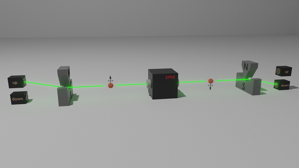
As it is a very famous quantum phenomenon, a lot has been written about entanglement in both the scientific and popular literature. However, it does still seem to be frequently misunderstood, with many surrounding misconceptions. I will attempt to explain the effects of entanglement in as straightforward a way as possible, with some very basic thought experiments. These can be followed without any understanding of what physical processes may be going on underneath. They only involve pressing a button on a box and observing the colour of a light bulb mounted on it. In fact, this is one of the features of quantum entanglement. It does not matter how you describe the physical world, whether you think of things as particles, waves, or whatever. Entanglement is an observable property independently of how, or even if, we try to describe the physical processes. Continue reading “Quantum Entanglement” →

The Khintchine Inequality

For a Rademacher sequence ${X=(X_1,X_2,\ldots)}$ and square summable sequence of real numbers ${a=(a_1,a_2,\ldots)}$ , the Khintchine inequality provides upper and lower bounds for the moments of the random variable,

$\displaystyle a\cdot X=a_1X_1+a_2X_2+\cdots.$

We use ${\ell^2}$ for the space of square summable real sequences and

$\displaystyle \lVert a\rVert_2=\left(a_1^2+a_2^2+\cdots\right)^{1/2}$

for the associated Banach norm.

Theorem 1 (Khintchine) For each ${0 < p < \infty}$ , there exists positive constants ${c_p,C_p}$ such that,

$\displaystyle c_p\lVert a\rVert_2^p\le{\mathbb E}\left[\lvert a\cdot X\rvert^p\right]\le C_p\lVert a\rVert_2^p,$ (1)

for all ${a\in\ell^2}$ .

Continue reading “The Khintchine Inequality” →

Rademacher Series

The Rademacher distribution is probably the simplest nontrivial probability distribution that you can imagine. This is a discrete distribution taking only the two possible values ${\{1,-1\}}$ , each occurring with equal probability. A random variable X has the Rademacher distribution if

$\displaystyle {\mathbb P}(X=1)={\mathbb P}(X=-1)=1/2.$

A Randemacher sequence is an IID sequence of Rademacher random variables,

$\displaystyle X = (X_1,X_2,X_3\ldots).$

Recall that the partial sums ${S_N=\sum_{n=1}^NX_n}$ of a Rademacher sequence is a simple random walk. Generalizing a bit, we can consider scaling by a sequence of real weights ${a_1,a_2,\ldots}$ , so that ${S_N=\sum_{n=1}^Na_nX_n}$ . I will concentrate on infinite sums, as N goes to infinity, which will clearly include the finite Rademacher sums as the subset with only finitely many nonzero weights.

Rademacher series serve as simple prototypes of more general IID series, but also have applications in various areas. Results include concentration and anti-concentration inequalities, and the Khintchine inequality, which imply various properties of ${L^p}$ spaces and of linear maps between them. For example, in my notes constructing the stochastic integral starting from a minimal set of assumptions, the ${L^0}$ version of the Khintchine inequality was required. Rademacher series are also interesting in their own right, and a source of some very simple statements which are nevertheless quite difficult to prove, some of which are still open problems. See, for example, Some explorations on two conjectures about Rademacher sequences by Hu, Lan and Sun. As I would like to look at some of these problems in the blog, I include this post to outline the basic constructions. One intriguing aspect of Rademacher series, is the way that they mix discrete distributions with combinatorial aspects, and continuous distributions. On the one hand, by the central limit theorem, Rademacher series can often be approximated well by a Gaussian distribution but, on the other hand, they depend on the discrete set of signs of the individual variables in the sum. Continue reading “Rademacher Series” →

Completions of *-Probability Spaces

We previously defined noncommutative probability spaces as a *-algebra together with a nondegenerate state satisfying a completeness property. Justification for the stated definition was twofold. First, an argument similar to the construction of measurable random variables on classical probability spaces was used, by taking all possible limits for which an expectation can reasonably be defined. Second, I stated various natural mathematical properties of this construction, including the existence of completions and their functorial property, which allows us to pass from preprobability spaces, and homomorphisms between these, to the NC probability spaces which they generate. However, the statements were given without proof, so the purpose of the current post is to establish these results. Specifically, I will give proofs of each of the theorems stated in the post on noncommutative probability spaces, with the exception of the two theorems relating commutative *-probability spaces to their classical counterpart (theorems 2 and 10), which will be looked at in a later post. Continue reading “Completions of *-Probability Spaces” →

Noncommutative Probability Spaces

In classical probability theory, we start with a sample space ${\Omega}$ , a collection ${\mathcal F}$ of events, which is a sigma-algebra on ${\Omega}$ , and a probability measure ${{\mathbb P}}$ on ${(\Omega,\mathcal F)}$ . The triple ${(\Omega,\mathcal F,{\mathbb P})}$ is a probability space, and the collection ${L^\infty(\Omega,\mathcal F,{\mathbb P})}$ of bounded complex-valued random variables on the probability space forms a commutative algebra under pointwise addition and products. The measure ${{\mathbb P}}$ defines an expectation, or integral with respect to ${{\mathbb P}}$ , which is a linear map

$\displaystyle \setlength\arraycolsep{2pt} \begin{array}{rl} &\displaystyle L^\infty(\Omega,\mathcal F,{\mathbb P})\rightarrow{\mathbb C},\smallskip\\ &\displaystyle X\mapsto{\mathbb E}[X]=\int X(\omega)d{\mathbb P}(\omega). \end{array}$

In this post I provide definitions of probability spaces from the algebraic viewpoint. Statements of some of their first properties will be given in order to justify and clarify the definitions, although any proofs will be left until later posts. In the algebraic setting, we begin with a *-algebra ${\mathcal A}$ , which takes the place of the collection of bounded random variables from the classical theory. It is not necessary for the algebra to be represented as a space of functions from an underlying sample space. Since the individual points ${\omega\in\Omega}$ constituting the sample space are not required in the theory, this is a pointless approach. By allowing multiplication of `random variables’ in ${\mathcal A}$ to be noncommutative, we incorporate probability spaces which have no counterpart in the classical setting, such as are used in quantum theory. The second and final ingredient is a state on the algebra, taking the place of the classical expectation operator. This is a linear map ${p\colon\mathcal A\rightarrow{\mathbb C}}$ satisfying the positivity constraint ${p(a^*a)\ge1}$ and, when ${\mathcal A}$ is unitial, the normalisation condition ${p(1)=1}$ . Algebraic, or noncommutative probability spaces are completely described by a pair ${(\mathcal A,p)}$ consisting of a *-algebra ${\mathcal A}$ and a state ${p}$ . Noncommutative examples include the *-algebra of bounded linear operators on a Hilbert space with pure state ${p(a)=\langle\xi,a\xi\rangle}$ for a fixed unit vector ${\xi}$ . Continue reading “Noncommutative Probability Spaces” →

The GNS Representation

As is well known, the space of bounded linear operators on any Hilbert space forms a *-algebra, and (pure) states on this algebra are defined by unit vectors. Considering a Hilbert space ${\mathcal H}$ , the space of bounded linear operators ${\mathcal H\rightarrow\mathcal H}$ is denoted as ${B(\mathcal H)}$ . This forms an algebra under the usual pointwise addition and scalar multiplication operators, and involution of the algebra is given by the operator adjoint,

$\displaystyle \langle x,a^*y\rangle=\langle ax,y\rangle$

for any ${a\in B(\mathcal H)}$ and all ${x,y\in\mathcal H}$ . A unit vector ${\xi\in\mathcal H}$ defines a state ${p\colon B(\mathcal H)\rightarrow{\mathbb C}}$ by ${p(a)=\langle\xi,a\xi\rangle}$ .

The Gelfand-Naimark–Segal (GNS) representation allows us to go in the opposite direction and, starting from a state on an abstract *-algebra, realises this as a pure state on a *-subalgebra of ${B(\mathcal H)}$ for some Hilbert space ${\mathcal H}$ .

Consider a *-algebra ${\mathcal A}$ and positive linear map ${p\colon\mathcal A\rightarrow{\mathbb C}}$ . Recall that this defines a semi-inner product on the *-algebra ${\mathcal A}$ , given by ${\langle x,y\rangle=p(x^*y)}$ . The associated seminorm is denoted by ${\lVert x\rVert_2=\sqrt{p(x^*x)}}$ , which we refer to as the ${L^2}$ -seminorm. Also, every ${a\in\mathcal A}$ defines a linear operator on ${\mathcal A}$ by left-multiplication, ${x\mapsto ax}$ . We use ${\lVert a\rVert_\infty}$ to denote its operator norm, and refer to this as the ${L^\infty}$ -seminorm. An element ${a\in\mathcal A}$ is bounded if ${\lVert a\rVert_\infty}$ is finite, and we say that ${(\mathcal A,p)}$ is bounded if every ${a\in\mathcal A}$ is bounded.

Theorem 1 Let ${(\mathcal A,p)}$ be a bounded *-probability space. Then, there exists a triple ${(\mathcal H,\pi,\xi)}$ where,

${\mathcal H}$ is a Hilbert space.

${\pi\colon\mathcal A\rightarrow B(\mathcal H)}$ is a *-homomorphism.

${\xi\in\mathcal H}$ satisfies ${p(a)=\langle\xi,\pi(a)\xi\rangle}$ for all ${a\in\mathcal A}$ .

${\xi}$ is cyclic for ${\mathcal A}$ , so that ${\{\pi(a)\xi\colon a\in\mathcal A\}}$ is dense in ${\mathcal H}$ .

Furthermore, this representation is unique up to isomorphism: if ${(\mathcal H^\prime,\pi^\prime,\xi^\prime)}$ is any other such triple, then there exists a unique invertible linear isometry of Hilbert spaces ${L\colon\mathcal H\rightarrow\mathcal H^\prime}$ such that

$\displaystyle \setlength\arraycolsep{2pt} \begin{array}{rl} &\displaystyle \pi^\prime(a)=L\pi(a)L^{-1},\smallskip\\ &\displaystyle \xi^\prime=L\xi. \end{array}$

Continue reading “The GNS Representation” →

Normal Maps

Given two *-probability spaces ${(\mathcal A,p)}$ and ${(\mathcal A^\prime,p^\prime)}$ , we want to consider maps ${\varphi\colon\mathcal A\rightarrow\mathcal A^\prime}$ . For example, we can look homomorphisms, which preserve the *-algebra operations, and can also consider restricting to state-preserving maps satisfying ${p^\prime(\varphi(a))=p(a)}$ . In algebraic probability theory, however, it is often necessary to include a continuity condition, leading to the idea of normal maps, which I look at in this post. In fact, as we will see, all *-homomorphisms between commutative probability spaces which preserve the state are normal, so this concept is most important in the noncommutative setting.

In contrast to the previous few posts on algebraic probability, the current post is a bit of a gear-change. We are still concerned with with the basic concepts of *-algebras and states. However, the main theorem stated below, which reduces to the Radon-Nikodym theorem in the commutative case, is deeper and much more difficult to prove than the relatively simple results with which I have been concerned with so far. Continue reading “Normal Maps” →

Operator Topologies

We previously defined the notion of positive linear maps and states on *-algebras, and noted that there always exists seminorms defining the ${L^2}$ and ${L^\infty}$ topologies. However, for applications to noncommutative probability theory, these are often not the most convenient modes of convergence to be using. Instead, the weak, strong, ultraweak and ultrastrong operator topologies can be used. This, rather technical post, is intended to introduce these concepts and prove their first properties.

Weak convergence on a *-probability space ${(\mathcal A,p)}$ is straightforward to define. A net ${a_\alpha\in\mathcal A}$ tends weakly to the limit ${a}$ if and only if ${p(xa_\alpha y)\rightarrow p(xay)}$ for all ${x,y\in\mathcal A}$ . Continue reading “Operator Topologies” →

Homomorphisms of *-Probability Spaces

I previously introduced the concept of a *-probability space as a pair ${(\mathcal A,p)}$ consisting of a state ${p}$ on a *-algebra ${\mathcal A}$ . As we noted, this concept is rather too simplistic to properly capture a noncommutative generalisation of classical probability spaces, and I will later give conditions for ${(\mathcal A,p)}$ to be considered as a true probability space. For now, I continue the investigation of these preprobability spaces, and will look at homomorphisms in this post.

A *-homomorphism between *-algebras ${\mathcal A}$ and ${\mathcal A^\prime}$ is a map ${\varphi\colon\mathcal A\rightarrow\mathcal A^\prime}$ preserving the algebra operations,

$\displaystyle \setlength\arraycolsep{2pt} \begin{array}{rl} &\displaystyle \varphi(\lambda a+\mu b)=\lambda\varphi(a)+\mu\varphi(b),\smallskip\\ &\displaystyle \varphi(ab)=\varphi(a)\varphi(b),\smallskip\\ &\displaystyle \varphi(a^*)=\varphi(a)^*, \end{array}$

for all ${a,b\in\mathcal A}$ and ${\lambda,\mu\in{\mathbb C}}$ . The term `*-homomorphism’ is used to distinguish it from the concept of simple algebra homomorphisms which need not preserve the involution (the third identity above). Next, I will say that ${\varphi}$ is a homomorphism of *-probability spaces ${(\mathcal A,p)}$ and ${(\mathcal A^\prime,p^\prime)}$ if it is a *-homomorphism from ${\mathcal A}$ to ${\mathcal A^\prime}$ which preserves the state,

$\displaystyle p^\prime(\varphi(a))=p(a),$

for all ${a\in\mathcal A}$ .

Now, recall that for any *-probability space ${(\mathcal A,p)}$ , we define a semi-inner product ${\langle x,y\rangle=p(x^*y)}$ on ${\mathcal A}$ and the associated ${L^2(p)}$ seminorm, ${\lVert x\rVert_2=\sqrt{p(x^*x)}}$ . Homomorphisms of *-probability spaces are clearly ${L^2}$ -isometries,

$\displaystyle \setlength\arraycolsep{2pt} \begin{array}{rl} \displaystyle \langle\varphi(x),\varphi(y)\rangle&\displaystyle=p^\prime\left(\varphi(x)^*\varphi(y)\right)=p^\prime\left(\varphi(x^*y)\right)\smallskip\\ &\displaystyle=p(x^*y)=\langle x,y\rangle. \end{array}$

For each ${a\in\mathcal A}$ , the ${L^\infty(p)}$ seminorm ${\lVert a\rVert_\infty}$ is defined as the operator norm of the left-multiplication map ${x\mapsto ax}$ on ${\mathcal A}$ , considered as a vector space with the ${L^2}$ seminorm. Homomorphisms of *-probability spaces do not need to be ${L^\infty}$ -isometric.

Lemma 1 If ${\varphi\colon(\mathcal A,p)\rightarrow(\mathcal A^\prime,p^\prime)}$ is a homomorphism of *-probability spaces then, for any ${a\in\mathcal A}$ ,

$\displaystyle \lVert\varphi(a)\rVert_\infty\ge\lVert a\rVert_\infty.$ (1)

Continue reading “Homomorphisms of *-Probability Spaces” →

	Anonymous on Spitzer’s Formula
	Anonymous on Spitzer’s Formula
	Anonymous on Brownian Bridges
	Anonymous on Spitzer’s Formula
	Anonymous on Spitzer’s Formula
	Anonymous on Spitzer’s Formula
	Anonymous on Spitzer’s Formula
	Anonymous on Spitzer’s Formula
	Anonymous on Spitzer’s Formula
	Anonymous on Spitzer’s Formula