Ito’s lemma is one of the most important and useful results in the theory of stochastic calculus. This is a stochastic generalization of the chain rule, or change of variables formula, and differs from the classical deterministic formulas by the presence of a quadratic variation term. One drawback which can limit the applicability of Ito’s lemma in some situations, is that it only applies for twice continuously differentiable functions. However, the quadratic variation term can alternatively be expressed using local times, which relaxes the differentiability requirement. This generalization of Ito’s lemma was derived by Tanaka and Meyer, and applies to one dimensional semimartingales.
The local time of a stochastic process X at a fixed level x can be written, very informally, as an integral of a Dirac delta function with respect to the continuous part of the quadratic variation ![{[X]^{c}}](https://s0.wp.com/latex.php?latex=%7B%5BX%5D%5E%7Bc%7D%7D&bg=ffffff&fg=000000&s=0&c=20201002) ,
,
![\displaystyle L^x_t=\int_0^t\delta(X-x)d[X]^c.](https://s0.wp.com/latex.php?latex=%5Cdisplaystyle++L%5Ex_t%3D%5Cint_0%5Et%5Cdelta%28X-x%29d%5BX%5D%5Ec.+&bg=ffffff&fg=000000&s=0&c=20201002) |
(1) |
This was explained in an earlier post. As the Dirac delta is only a distribution, and not a true function, equation (1) is not really a well-defined mathematical expression. However, as we saw, with some manipulation a valid expression can be obtained which defines the local time whenever X is a semimartingale.
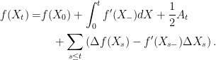
Going in a slightly different direction, we can try multiplying (1) by a bounded measurable function  and integrating over x. Commuting the order of integration on the right hand side, and applying the defining property of the delta function, that
 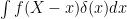 is equal to
  , gives
![\displaystyle \int_{-\infty}^{\infty} L^x_t f(x)dx=\int_0^tf(X)d[X]^c.](https://s0.wp.com/latex.php?latex=%5Cdisplaystyle++%5Cint_%7B-%5Cinfty%7D%5E%7B%5Cinfty%7D+L%5Ex_t+f%28x%29dx%3D%5Cint_0%5Etf%28X%29d%5BX%5D%5Ec.+&bg=ffffff&fg=000000&s=0&c=20201002) |
(2) |
By eliminating the delta function, the right hand side has been transformed into a well-defined expression. In fact, it is now the left side of the identity that is a problem, since the local time was only defined up to probability one at each level x. Ignoring this issue for the moment, recall the version of Ito’s lemma for general non-continuous semimartingales,
 |
(3) |
where ![{A_t=\int_0^t f^{\prime\prime}(X)d[X]^c}](https://s0.wp.com/latex.php?latex=%7BA_t%3D%5Cint_0%5Et+f%5E%7B%5Cprime%5Cprime%7D%28X%29d%5BX%5D%5Ec%7D&bg=ffffff&fg=000000&s=0&c=20201002) . Equation (2) allows us to express this quadratic variation term using local times,
. Equation (2) allows us to express this quadratic variation term using local times,
The benefit of this form is that, even though it still uses the second derivative of  , it is only really necessary for this to exist in a weaker, measure theoretic, sense. Suppose that is convex, or a linear combination of convex functions. Then, its right-hand derivative
  exists, and is itself of locally finite variation. Hence, the Stieltjes integral
  exists. The infinitesimal
  is alternatively written
  and, in the twice continuously differentiable case, equals
  . Then,
 |
(4) |
Using this expression in (3) gives the Ito-Tanaka-Meyer formula. Continue reading “The Ito-Tanaka-Meyer Formula” →


-Hölder continuous w.r.t. x, for all
and over all bounded regions for t.


 between metric spaces E and F is said to be
 . The smallest value of C satisfying this inequality is known as the
  , then every
  -Hölder continuous map from E is also
  -Hölder continuous. In particular, 1-Hölder and Lipschitz continuity are equivalent.
 are almost surely locally Hölder continuous. That is, they are almost surely Hölder continuous on every bounded interval. To start with, we look at real-valued processes. Throughout this post, we work with repect to a probability space
  . There is no need to assume the existence of any filtration, since they play no part in the results here
 be a real-valued stochastic process such that there exists positive constants
  satisfying
 ![\displaystyle {\mathbb E}\left[\lvert X_t-X_s\rvert^\alpha\right]\le C\lvert t-s\vert^{1+\beta},](https://s0.wp.com/latex.php?latex=%5Cdisplaystyle++%7B%5Cmathbb+E%7D%5Cleft%5B%5Clvert+X_t-X_s%5Crvert%5E%5Calpha%5Cright%5D%5Cle+C%5Clvert+t-s%5Cvert%5E%7B1%2B%5Cbeta%7D%2C+&bg=ffffff&fg=000000&s=0&c=20201002)
 . Then, X has a continuous modification which, with probability one, is locally
  .
. 
 and
and  be finite measure spaces, and
  be a bounded
  -measurable function. Then,
 -measurable,
 -measurable, and,
 .
.


![{[S]_\infty}](https://s0.wp.com/latex.php?latex=%7B%5BS%5D_%5Cinfty%7D&bg=ffffff&fg=000000&s=0&c=20201002)
![[S]_\infty](https://s0.wp.com/latex.php?latex=%5BS%5D_%5Cinfty&bg=ffffff&fg=000000&s=0&c=20201002)
![[S]](https://s0.wp.com/latex.php?latex=%5BS%5D&bg=ffffff&fg=000000&s=0&c=20201002)

